The Post-Glacial Flooding Hypothesis – 1/11

Posted on August 14, 2026 by admin

Chapter 1 – The Legacy of the Ice Age

Book Extract

1. Introduction

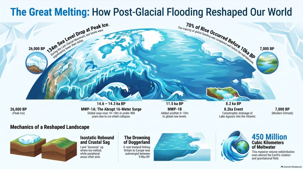
Roughly twenty-six thousand years ago, the Earth entered the final phase of the last ice age, when more than 30 million square kilometres of the northern continents were mantled by ice. Sea level dropped by over a hundred metres, continents expanded, and the atmosphere became drier and dustier. When the climate warmed, that frozen water returned to the ocean basins, transforming every river and shoreline on the planet. Understanding the magnitude and tempo of this transition is fundamental to reconstructing the landscapes that Holocene societies inherited. (The Post-Glacial Flooding Hypothesis)

The scientific history of sea-level research stretches back more than a century. Fairbridge (1961) first proposed that global “drowned terraces” recorded former sea levels. Oxygen-isotope analysis later provided a direct measure of global ice volume (Shackleton & Opdyke 1973; Chappell & Shackleton 1986). By the 1990s, uranium-thorium dating of coral reefs (Bard et al., 1990) and glacio-isostatic models (Lambeck & Chappell 2001) produced continuous global sea-level curves for the late Quaternary. Satellite altimetry and GRACE gravimetry now track present-day mass exchange between ice sheets and oceans with millimetre precision (Watkins et al., 2015; Cazenave et al., 2018).

These cumulative datasets reveal that the transformation from the Last Glacial Maximum (LGM) to the modern interglacial was neither instantaneous nor globally uniform. The following sections examine the evidence for the magnitude of the LGM, the deglacial rise in sea level, and the feedbacks that coupled ice, ocean, and atmosphere into a single dynamic system.

2. The Last Glacial Maximum

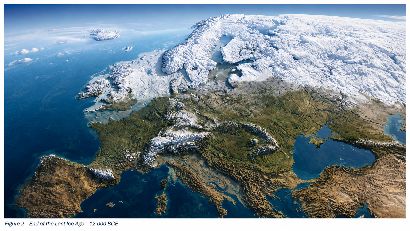
The LGM, dated between ~26 000 and 19 000 years BP, represents the maximum combined extent of Northern Hemisphere ice sheets. Reconstructions by Ehlers et al. (2018) show the Laurentide Ice Sheet extending south of the Great Lakes, the Fennoscandian complex covering Scandinavia, northern Britain, and the Baltic, and separate domes over the Barents and Kara Seas. In the Southern Hemisphere, the Patagonian, New Zealand, and Antarctic ice sheets expanded simultaneously. Global mean air temperature was about 5–6 °C lower than today (Tierney et al., 2020).

Cosmogenic-nuclide dating of moraines indicates near-synchronous maxima in both hemispheres within 1–2 kyr (Balco et al., 2009). Ice cores from Antarctica record atmospheric CO₂ concentrations of only ~190 ppm, the lowest of the last 800 kyr (Lüthi et al., 2008). The increased planetary albedo and reduced greenhouse forcing locked the Earth into a radiative imbalance until orbital precession increased summer insolation at high latitudes around 21 ka BP, initiating melting.

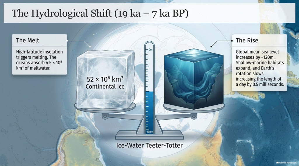
Sea level at the LGM stood 134 ± 5 m below present (Rohling et al., 2009; Lambeck et al., 2014), implying an extra ~52 × 10⁶ km³ of continental ice—roughly triple modern Antarctic volume. The load depressed the lithosphere by up to a kilometre and generated a peripheral forebulge hundreds of kilometres wide. When deglaciation began, these distortions created regional variations in relative sea level (RSL) of tens of metres—a problem that still complicates correlation between sites.

3. Quantifying Global Ice and Sea-Level Change

High-resolution oxygen-isotope records from the Red Sea (Rohling et al., 2009) and global benthic stacks (Lisiecki & Raymo, 2005) define the eustatic component of sea-level change. Grant et al. (2014) extended the Red Sea curve to 500 kyr BP and confirmed an approximately linear relation between δ¹⁸O and global mean sea level within ±140 m. Combined with coral-reef U/Th dates (Peltier & Fairbanks 2006) and glacio-isostatic modelling (ICE-6G v2; Peltier et al., 2015), these data yield the following deglacial sequence:

Stable minimum (26–19 ka) — Sea level constant near −130 m; ice volume at maximum.
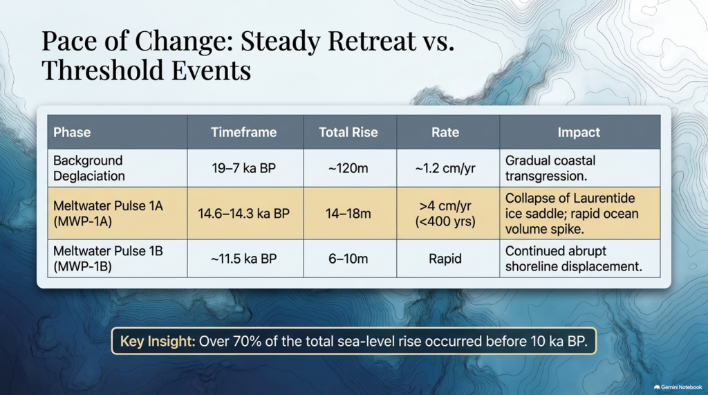
Deglacial rise (19–7 ka) — Global mean increase ~120 m; average rate ~1.2 cm yr⁻¹.

Waelbroeck et al. (2019) and Gowan et al. (2021) further improved resolution, showing that roughly 70% of the total rise occurred before 10 ka BP and that rates exceeded 4 cm yr⁻¹ during short meltwater pulses. These figures quantify the pace of global hydrological reorganisation that followed the LGM.

4. Meltwater Pulses and Deglacial Chronology

Superimposed on the long-term trend are several abrupt accelerations known as Meltwater Pulses (MWPs). MWP-1A (14.6–14.3 ka BP) raised global sea level by 14–18 m in < 400 years (Deschamps et al., 2012). Coral cores from Tahiti and Barbados capture the event as a distinct change in growth depth and isotope composition. MWP-1B, centred near 11.5 ka BP, added another 6–10 m (Liu et al., 2019). A later, smaller pulse (~8.2 ka BP) corresponded to catastrophic drainage of pro-glacial Lake Agassiz into the North Atlantic (Teller et al., 2002).

Numerical models (Gregoire et al., 2012) indicate that collapse of the Laurentide ice saddle triggered MWP-1A, releasing freshwater at ~0.3 Sverdrups—enough to disrupt the Atlantic Meridional Overturning Circulation (AMOC) and cause short-lived cooling across the Northern Hemisphere (Liu et al., 2009). Geomorphic evidence of megafloods, such as the Missoula outburst channels in North America (Bretz 1969; Baker 2013), provides analogues for the required discharge scale.

MWPs demonstrate that deglaciation was a series of threshold events rather than a steady retreat. The timing of pulses aligns closely with abrupt climatic shifts seen in Greenland ice cores (NGRIP Members 2004), underscoring the tight coupling between ice dynamics and global climate.

5. Isostatic Rebound and Crustal Adjustment

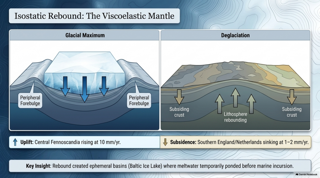
Once surface loads were removed, the lithosphere began to rebound. The process is governed by viscoelastic relaxation of the mantle with characteristic times of 1–5 kyr (Milne et al., 2006). Modern GPS and tide-gauge data show uplift of 10 mm yr⁻¹ in central Fennoscandia and subsidence of 1–2 mm yr⁻¹ in southern England and the Netherlands—the collapsing forebulge. Modelling (Lambeck et al., 2014; Peltier et al., 2015) reproduces these patterns when mantle viscosities of 3–5 × 10²¹ Pa s are used.

Rebound created ephemeral basins along glacial margins where meltwater ponded before marine incursion. The Baltic Ice Lake and the Champlain Sea are classic examples, forming as differential uplift temporarily dammed drainage routes (Saarnisto & Salonen 1995; Parent & Occhietti 1999). Many present-day estuaries owe their origins to these basins. Sediment cores from the Humber, Thames, and Rhine estuaries contain alternating freshwater and brackish layers that track the balance between isostasy and eustasy (Shennan et al., 2018).

6. The Rebirth of the Oceans

Between 19 ka and 7 ka BP, the oceans absorbed roughly 4.5 × 10⁸ km³ of meltwater, raising mean sea level by ~120 m. Coral records from Tahiti, Huon Peninsula, and the Sunda Shelf show a remarkably consistent transgression curve (Deschamps et al., 2012; Hanebuth et al., 2000). By 7 ka BP, sea level stabilised within a few metres of the modern datum.

The redistribution of this mass altered Earth’s rotation and gravitational field, increasing the length of day by 0.5 milliseconds (Mitrovica & Munk 2003) and displacing the geoid by several decimetres. More tangibly, flooding of continental shelves expanded shallow-marine habitats and enhanced nutrient exchange between land and sea, fuelling mid-Holocene marine productivity (Haug et al., 2001). The creation of new estuarine and lagoonal systems also provided nursery grounds for species that later became critical to human subsistence.

7. Climate Feedbacks During Deglaciation

Ice-core and modelling studies reveal that the deglacial rise in greenhouse gases both responded to and accelerated warming. CO₂ increased from 190 ppm at the LGM to 270 ppm by 11 ka BP (Lüthi et al., 2008). Methane doubled from 350 to 700 ppb (Loulergue et al., 2008). The combined radiative forcing of ~2.5 W m⁻² produced a global temperature increase of ~4 °C (IPCC AR6 2021). Shakun et al. (2012) demonstrated that Antarctic warming led the CO₂ rise by several centuries, implying that oceanic outgassing initiated the feedback loop.

Freshwater discharges into the North Atlantic weakened the AMOC and triggered millennial-scale climate reversals. The Younger Dryas (12.9–11.7 ka BP) involved a 5–7 °C drop in Greenland temperatures followed by rapid recovery within a few decades (Severinghaus et al., 1998). Numerical experiments show that such shifts require freshwater fluxes of 0.05–0.1 Sverdrups (Liu et al., 2009). Once meltwater routing shifted southward and AMOC strength recovered, interglacial stability was achieved.

8. The Transformation of North-West Europe

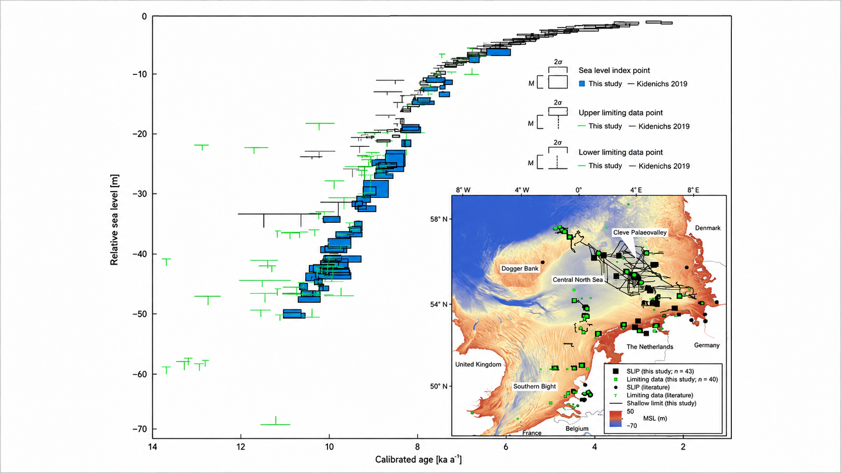
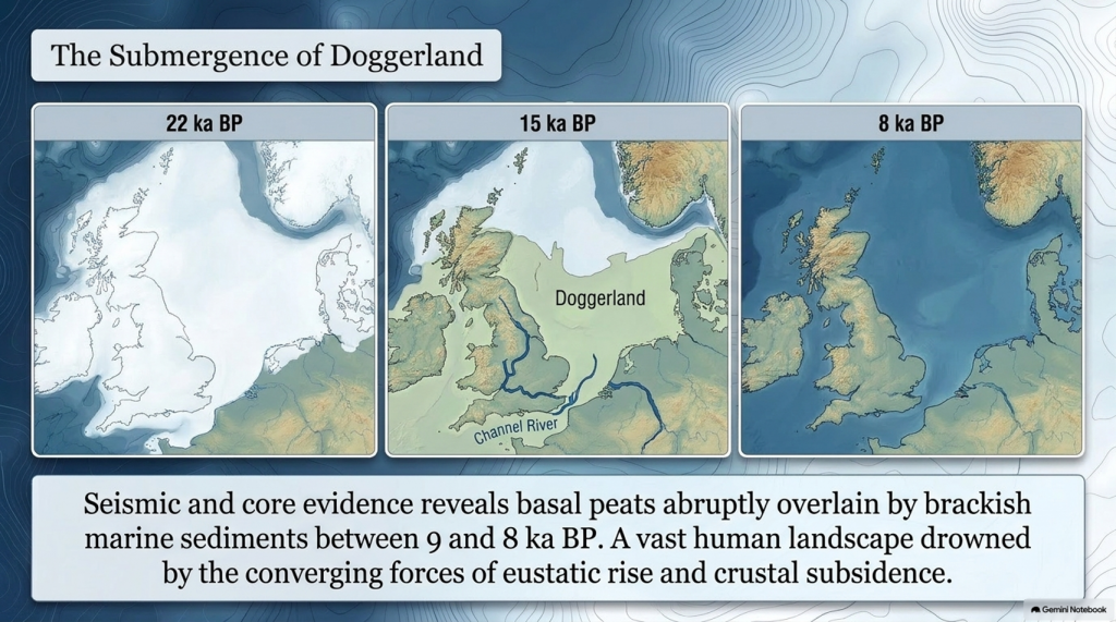
Retreat of the British–Irish Ice Sheet began near 22 ka BP and concluded by 15 ka BP (Clark et al., 2012). Deglaciation exposed outwash plains and periglacial lakes that evolved into estuaries and wetlands as sea level rose. Seismic and core evidence from the southern North Sea shows basal peats overlain by brackish and marine sediments between 9 and 8 ka BP (Hijma & Cohen 2011). These sequences chart the drowning of Doggerland—a vast lowland linking Britain to Europe. Pollen and macrofossil data indicate temperate woodland colonisation prior to submergence (Gaffney et al., 2009).

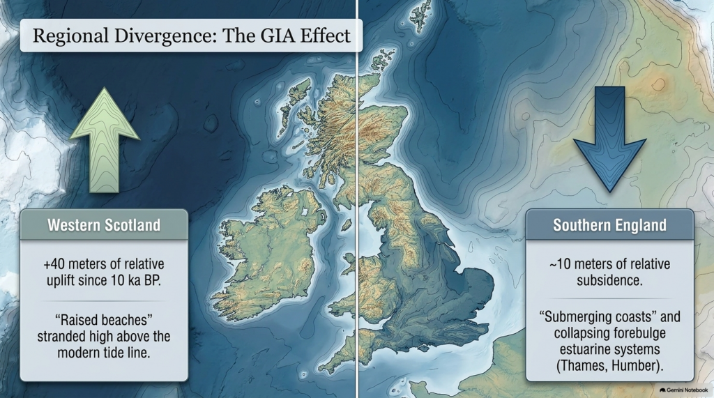
Regional RSL curves diverge sharply due to GIA: western Scotland has risen > 40 m since 10 ka, while southern England has subsided by ~10 m (Bradley et al., 2020). Raised beaches in the north and submerged forests in the south reflect this differential motion. In the English Channel, fluvial erosion during early deglaciation carved the “Channel River,” later flooded by 8 ka (Mellett et al., 2013). Similar sequences occur along the Irish and Danish coasts, documenting the progressive marine transgression of northwest Europe.

9. Towards a Global–Regional Synthesis

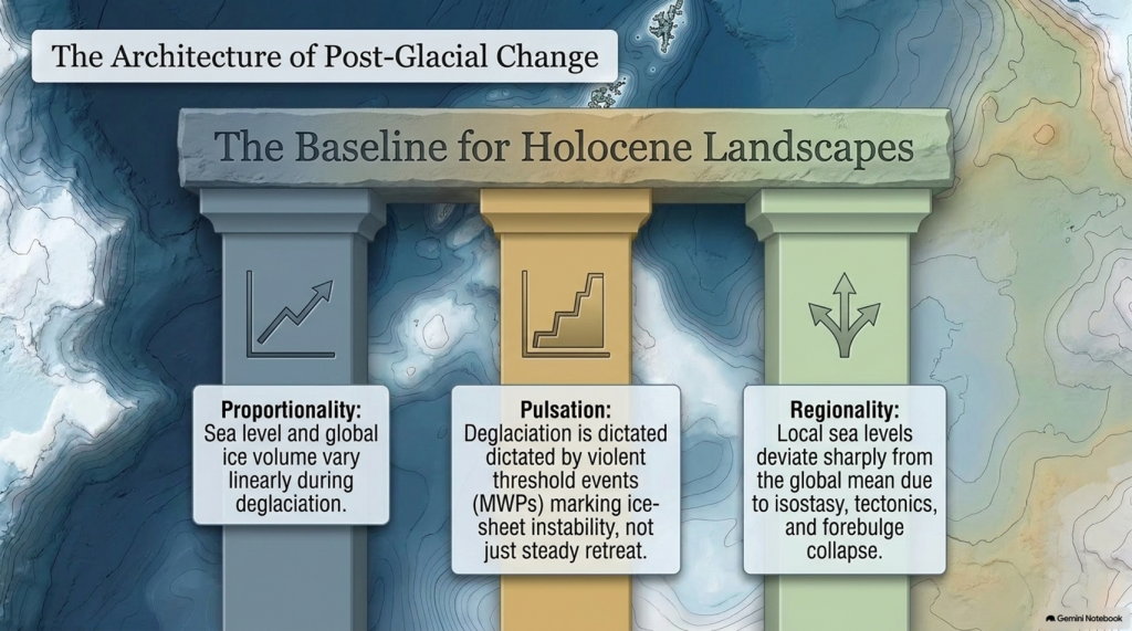
By combining isotopic, coral, and geodetic datasets, modern reconstructions achieve decimetre precision for Holocene sea level (Gowan et al., 2021). Three principles emerge:

Proportionality — Sea level and global ice volume vary linearly during deglaciation.
Pulsation — Superimposed meltwater pulses mark thresholds in ice-sheet stability.
Regionality — Local deviations result from isostasy, tectonics, and sediment compaction.

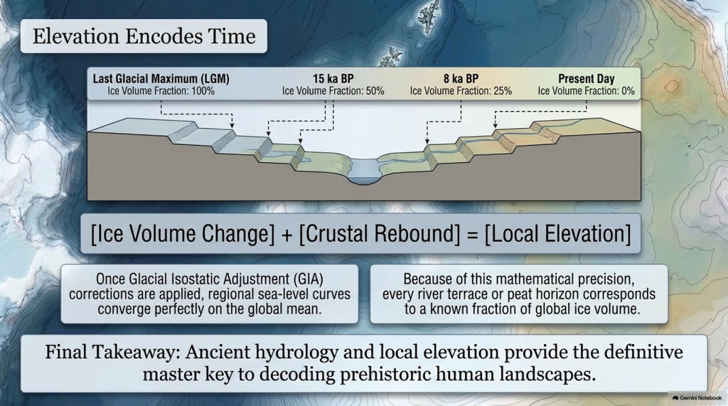
Shennan et al. (2018) synthesised over 500 Holocene RSL indicators for the British Isles, demonstrating that once GIA corrections are applied, regional curves converge on the global mean within analytical error. These findings provide a quantitative baseline for analysing river-terrace altitudes and groundwater histories in later chapters.

Equally important, comparison with modern sea-level observations highlights the extraordinary pace of contemporary change. Satellite altimetry records a mean rise of 3.4 ± 0.4 mm yr⁻¹ since 1993 (Cazenave et al., 2018)—an order of magnitude faster than the late-Holocene background rate (Kopp et al., 2016). The processes that ended the last ice age therefore remain relevant to current climate dynamics.

10. Conclusion

The end of the last ice age was a planetary event in which ice, water, and rock interacted on colossal scales. Between 26 ka and 7 ka BP, sea level rose more than 120 m, ice sheets vanished from most temperate latitudes, and the hydrological cycle intensified. The evidence—oxygen-isotope curves, coral terraces, basal peats, and glacio-isostatic models—forms a coherent narrative of gradual yet punctuated change.

These quantitative reconstructions define the environmental backdrop for all Holocene landscapes. They also establish a principle crucial to later chapters: that elevation within fluvial and coastal systems encodes time, because each terrace or peat horizon corresponds to a known fraction of global ice volume. The following chapter therefore turns from global physics to the mathematical description of flooding itself—the equations that translate ice-volume change into measurable hydrological response.

Plain-Language Conclusion

The ice age was like the planet putting a huge amount of the world’s water into giant freezers on land. When those freezers started to melt:

All that stored water went back into the oceans.
The seas rose by about 120 metres.
The weight of the ice came off the land, so some places bounced up, others sagged down.

Scientists can see this story in:

tiny shells on the sea floor,
old coral reefs now sitting at the “wrong” depths,
layers of mud and peat around coasts.

Put simply:

We froze the oceans on land, then poured them back in. The combination of rising seas and bouncing crust rearranged coastlines everywhere, and we can measure it.

To read the rest of the book, follow this link: https://prehistoric-britain.co.uk/the-post-glacial-flooding-hypothesis-book

FREE ONLINE BOOK is available HERE: https://prehistoric-britain.co.uk/the-post-glacial-flooding-hypothesis-book

PODCAST

Author’s Biography

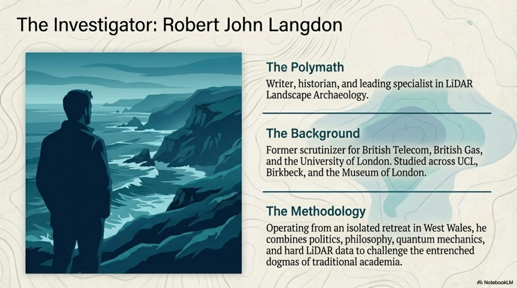
Robert John Langdon, a polymathic luminary, emerges as a writer, historian, and eminent specialist in LiDAR Landscape Archaeology.

His intellectual voyage has been interwoven with stints as an astute scrutineer in government and grand corporate bastions, a tapestry spanning British Telecommunications, Cable and Wireless, British Gas, and the esteemed University of London.

A decade hence, Robert’s transition into retirement unfurled a chapter of insatiable curiosity. This phase saw him immerse himself in Politics, Archaeology, Philosophy, and the enigmatic realm of Quantum Mechanics. His academic odyssey traversed the venerable corridors of knowledge hubs such as the Museum of London, University College London, Birkbeck College, The City Literature Institute, and Chichester University.

In the symphony of his life, Robert is a custodian of three progeny and a pair of cherished grandchildren. His sanctuary lies ensconced in the embrace of West Wales, where he inhabits an isolated cottage, its windows framing a vista of the boundless sea – a retreat from the scrutinising gaze of Her Majesty’s Revenue and Customs, an amiable clandestinity in the lap of nature.

Exploring Prehistoric Britain: A Journey Through Time

My blog delves into the fascinating mysteries of prehistoric Britain, challenging conventional narratives and offering fresh perspectives grounded in cutting-edge research, particularly LiDAR technology. I invite you to explore some key areas of my research. For example, the Wansdyke, often cited as a defensive structure, is re-examined in light of new evidence. I’ve presented my findings in my blog post Wansdyke: A British Frontier Wall – ‘Debunked’, and a Wansdyke LiDAR Flyover video further visualises my conclusions.

My work also often challenges established archaeological dogma. I argue that many sites, such as Hambledon Hill, commonly identified as Iron Age hillforts, are not what they seem. My posts Lidar Investigation Hambledon Hill – NOT an ‘Iron Age Fort’ and Unmasking the “Iron Age Hillfort” Myth explore these ideas in detail and offer an alternative view. Similarly, sites like Cissbury Ring and White Sheet Camp receive re-evaluations based on LiDAR analysis in my posts “Lidar Investigation Cissbury Ring through time” and “Lidar Investigation White Sheet Camp,“ revealing fascinating insights into their true purpose. I have also examined South Cadbury Castle, often linked to the mythical Camelot56.

My research also extends to ancient water management, including the role of canals and other linear earthworks. I have discussed the true origins of Car Dyke in multiple posts, including Car Dyke – ABC News Podcast and Lidar Investigation Car Dyke – North Section, which suggest a Mesolithic origin 2357. I also explore the misidentification of Roman aqueducts, as seen in my posts on the Great Chesters (Roman) Aqueduct. My research has also been greatly informed by my post-glacial flooding hypothesis, which has helped explain landscape transformations over time. I have discussed this hypothesis in several posts, including AI now supports my Post-Glacial Flooding Hypothesis and Exploring Britain’s Flooded Past: A Personal Journey

Finally, my blog also investigates prehistoric burial practices, as seen in Prehistoric Burial Practices of Britain and explores the mystery of Pillow Mounds, often mistaken for medieval rabbit warrens, but with a potential link to Bronze Age cremation in my posts: Pillow Mounds: A Bronze Age Legacy of Cremation? and The Mystery of Pillow Mounds: Are They Really Medieval Rabbit Warrens?. My research also includes astronomical insights into ancient sites, for example, in Rediscovering the Winter Solstice: The Original Winter Festival. I also review new information about the construction of Stonehenge in The Stonehenge Enigma.

Archaeology in the Post-Truth Era

Posted on April 6, 2026 by admin

Introduction

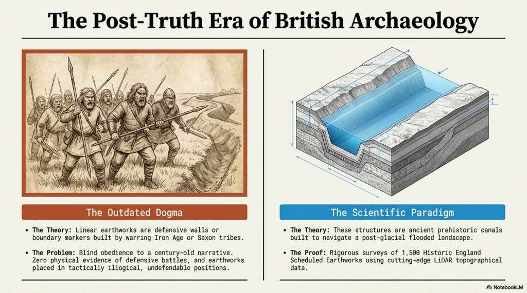
Over the past ten years, I’ve faced a constant uphill battle to establish what I consider a straightforward conclusion—that Linear Earthworks are not defensive structures or boundary markers but prehistoric canals. It’s a claim that’s been dismissed repeatedly, often without proper engagement, but that resistance never stopped the work.(Archaeology in the Post-Truth Era)

Instead, it pushed me further. I carried out a full survey of over 1,500 of Historic England’s Scheduled Linear Earthworks, systematically analysing their form, placement, and context. That work eventually led to the first book in what has now become a larger series, focusing specifically on the East Wansdyke area. For me, that publication wasn’t just another book—it was a milestone. It represents a level of detailed, landscape-wide analysis that, to date, no university or research team has attempted at this scale.

(Britain's Giant Prehistoric Waterways) — Archaeology in the Post-Truth Era

The book itself takes a forensic approach. Every aspect of East Wansdyke is examined and placed into a wider framework—what I define as an ancient prehistoric canal system. The aim is simple: to challenge the existing archaeological narrative, not with speculation, but with measurable, testable evidence. The traditional explanations—defensive lines, territorial markers—don’t hold up under scrutiny. They lack physical evidence, contradict their own logic, and fail to explain the most basic characteristics of these structures.

What emerges instead is something far more significant. If these earthworks are canals, then we are looking at a completely different level of engineering capability in prehistory. These were not crude societies marking out land or preparing for war—they were shaping landscapes, managing water, and building infrastructure on a national scale. This not only challenges the archaeological community but also opens the door to a broader re-evaluation of how prehistoric landscapes were understood and used.

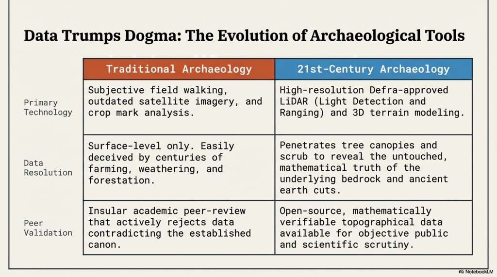
Embarking on this journey was not without its challenges, especially in an era where scepticism often overshadows scientific evidence. The response to my publication, which I had hoped would ignite a meaningful academic debate, was instead largely silent. Despite the use of modern LiDAR technology and a dataset far beyond what had previously been attempted, the work was either ignored or dismissed as speculative.

This resistance was mirrored on social media, where entrenched views dominated discussion. Any attempt to challenge established narratives was met with denial rather than engagement. Peer review, rather than being treated as part of an evolving process, was often presented as a final and unquestionable authority.

The Dyke Myth Collapse — Archaeology in the Post-Truth Era

This kind of blind adherence to established ideas is not unique to archaeology. It is a pattern repeated across disciplines, where existing frameworks are protected rather than tested. New evidence is not examined on its merits but rejected because it disrupts the accepted model.

That was the position in 2014.

Now, two years on, we can assess that position against new evidence—and, more importantly, against the predictions made at the time.

What has emerged since then is not a contradiction of the original work, but a direct reinforcement of it.

The borehole data, when analysed correctly using elevation rather than arbitrary depth, has revealed consistent clustering of water-related deposits at specific heights across multiple independent locations. Statistically, this pattern is highly unlikely to occur by chance and instead points to a structured, elevation-controlled hydrological system operating across the landscape.

At the same time, the mathematical framework behind the Post-Glacial Flooding Hypothesis has continued to develop. The mass-balance calculations, combined with ice-volume scaling and groundwater discharge modelling, demonstrate that Britain remained in a prolonged state of elevated water tables and enlarged river systems for thousands of years after the end of the last Ice Age.

This confirms a critical point:

The rivers of the past were higher than those we see today.

And once that is understood, the entire interpretation of Linear Earthworks shifts.

Rethinking The Past — Archaeology in the Post-Truth Era

Because these structures are not randomly placed. They align with contours, connect basins, and sit within hydrological positions that make sense only under sustained high water levels. Their form, scale, and distribution are consistent with water management—not defence, not boundaries, but controlled flow.

In other words, the environmental conditions required for canals are now demonstrably present.

This is the key difference between 2014 and 2026.

In 2014, the argument was based on landscape logic, structural analysis, and comparative reasoning.

In 2026, that same argument is now supported by independent physical data and mathematical proof of the environmental conditions required for it to function.

The conclusion, however, has not changed.

Linear Earthworks were constructed in a landscape defined by elevated water tables and expanded river systems. Within that context, their most coherent and evidence-based interpretation remains exactly what was originally proposed.

They were canals.

And perhaps most importantly, this progression follows the correct scientific sequence.

The prediction came first.

The evidence followed.

And that is not speculation—that is validation.

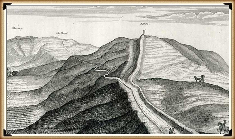
Wansdyke

In my book, I meticulously addressed every single meter of East Wansdyke, providing compelling evidence that challenges the traditional interpretation of Wansdyke as either a defensive structure or a boundary marker. My research and analysis have convincingly demonstrated that East Wansdyke was, in fact, part of a prehistoric canal system, a finding that significantly alters our understanding of the landscape and the capabilities of the people who engineered it. This conclusion was reached through a combination of detailed survey work, the application of modern technologies such as LiDAR, and a critical review of the archaeological and historical records.

However, one critic, emblematic of the resistance I’ve encountered, sought to undermine my hypothesis by citing a site associated with West Wansdyke. This individual argued that because West Wansdyke was built on a ‘late Iron Age’ fortification, it must, therefore, be of Saxon origin, aiming to cast doubt on my entire thesis by focusing on this one aspect. It’s a classic example of attempting to discredit a comprehensive theory by finding fault with a single, arguably tangential, element.

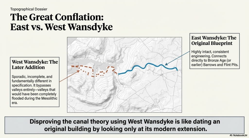
In my response, I emphasised that this site, situated in West Wansdyke, falls outside the primary focus of my research on the East Wansdyke segment. More importantly, I had already anticipated such objections and addressed them directly in my book. I concluded that West Wansdyke, while geographically related, was connected to the original canal system at a later date, likely by the Romans. This connection was based on evidence suggesting that West Wansdyke is incomplete, sporadic, and differs in specification from East Wansdyke, indicating a distinct phase of construction and purpose.

The dismissal of West Wansdyke from my primary analysis was not arbitrary but a considered decision grounded in the evidence and the scope of my research. It reflects a methodological approach that prioritises coherence, specificity, and relevance in building a historical narrative. The critique of my work that focuses on West Wansdyke, therefore, misses the mark. It overlooks the rigour of my research process and the clear rationale provided for the conclusions drawn about East Wansdyke and its role within a broader prehistoric canal system.

This encounter serves as a reminder of the challenges inherent in advancing new theories in archaeology, especially those that significantly depart from established interpretations. It also underscores the importance of clarity, precision, and thoroughness in both research and communication, qualities I strived to embody in my work on East Wansdyke.

West Wansdyke

We have a problem with West Wansdyke – it’s not part of East Wansdyke. This has always been a historical debate over the last 100 years. If we look at the limited archaeological evidence, we find that although it may have been a much later Canal/Dyke it is not contemporary with the East Wansdyke canal and was not built at the same time.

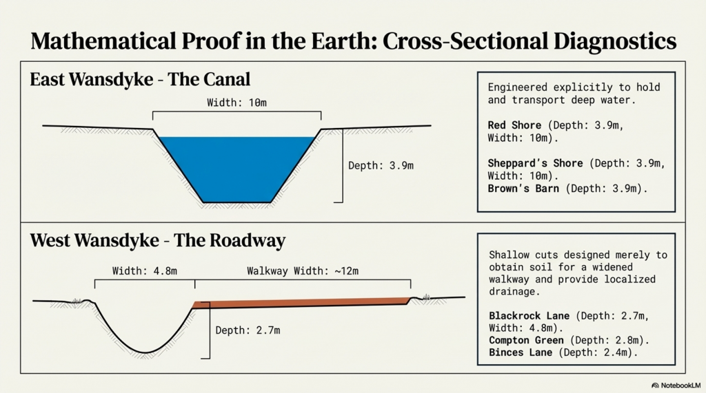
Excavations conclusively show that the Ditches on the East side of Wansdyke are much more profound and twice as broad. In contrast, the Banks on the East Side are much wider. We see that East Dyke was built first, as our River height model shows that most of West Wansdyke would have been flooded or marshland at the time of use.

Location	Wansdyke
Bank	Ditch	Excavator notes
Materials	Width	Height	Berm	Width	Depth	Counterscarp
EAST
Red Shore	Clay/Flints	9.5	2	N	10	3.9	Y	Green 1966
Sheppard’s shore		10	2.3	N	10	3.9	Y	Pitt Rivers 1888
Brown’s Barn		9	2.3	N	10	3.9	Y	Pitt Rivers 1891
WEST
Binces Lane West	Stoney	12.5	??	??	3.5	1.7	Y	Erskine 1990s
Binces Lane East	Stoney	?	5?	N	6	2.4	?	Erskine 1990s
Compton Green	Clay marl	13	0.8	Y	5.8	2.8	Y	Erskine 1990s
Blackrock Lane	Silty Clay	12.5	1.7	Y	4.8	2.7	?	Erskine 1990s
Park farm	Stones	10	0.4	Y	5.5	2.4	Y	Erskine 1990s
Fairy Hill		13	?	Y	6.5	?		Erskine 1990s

West Wansdyke Excavation

When the waters receded (possibly Early Iron Age period), it is possible that the Dyke was extended, or the more probable event of East Wansdyke after it dried up was turned into a roadway and what we see in West Wansdyke is the extension of the road, and hence it is wider than in the East.

We also see more shallow ditches as they were not used for water but to obtain soil for the walkway and become drainage ditches.

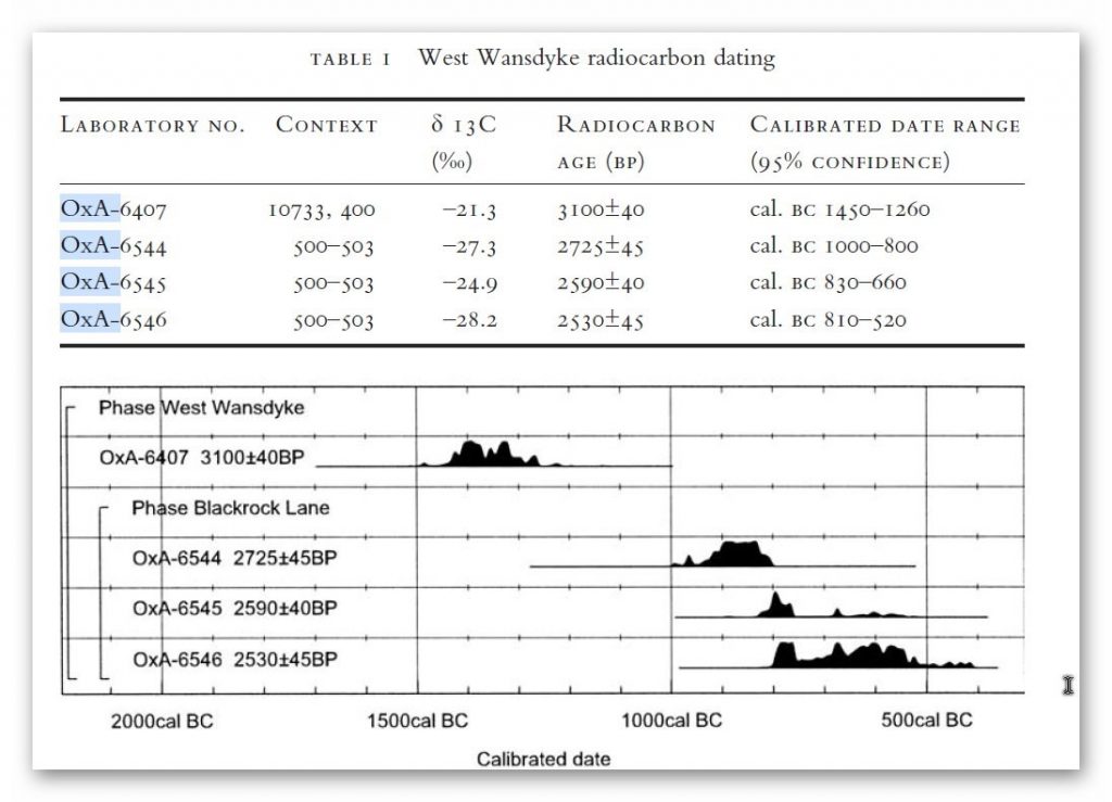
Indeed, we know the Romans used this as a road and always had drainage ditches, usually on both sides. This is supported by carbon dating at Erskine’s excavation at Blackrock Lane, where the section appeared to have been sealed by the primary bank material. One of these layers contained significant concentrations of woody oak charcoal.

Samples of this material were submitted to the Ancient Monuments Laboratory for radiocarbon dating to provide a possible construction of the bank. Unfortunately, as shown in the table below – sadly, as standard when scientific evidence disproves the current archaeological narrative – it is ignored and classified as an error.

Table 1. Erskine, Jonathan. (2007). The West Wansdyke: an appraisal of the dating, dimensions and construction techniques in the light of excavated evidence. Archaeological Journal. 164. 80-108.

The other missing aspect, shown in East Wansdyke but not in West Wansdyke, was the massive connection to Barrows and Flint Pits. Again, this connection is not seen on West Wansdyke, which may help date this monument, as the barrows were of the Bronze Age or earlier, and, as we have seen from the carbon dating evidence at Blackrock Lane, much earlier than its 1500 BCE date.

Statonbury Camp near Bath – an example of West Wansdyke

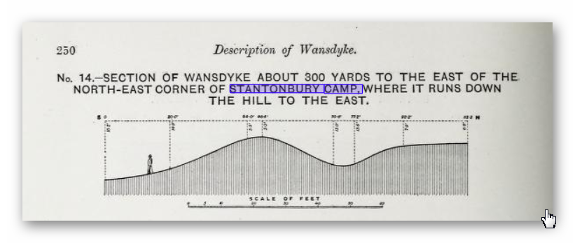
If we look at the Scheduled parts of the Wansdyke – we see that the East is very much intact, but the West is sporadic at best, and it’s hard to find a logical link to all the Dykes that seem to only appear over hills and not in the valley’s – which in my view would have been flooded in the Mesolithic and hence the west sections addition after East Wansdyke’s construction – probably by the roman’s who may have utilised the Dyke system for their own transportation reasons. But for the sake of scientific curiosity, let’s take a detailed look at Stantonbury Hill site, which is classified as an Iron Age Camp, with Wansdyke making up one of the defensive banks – but before we delve deeper into the field archaeology of the site – I feel I must clarify the use of the classification of ‘Iron Age Fort’ by archaeologists.

All sites that sit on top of hills and have ditches are called Iron Age Forts – sadly, I have yet to find a single location that is either ‘Iron Age’ or a ‘Fortification’, as not a single dead body from slaying has ever been found, and all the so-called defensive ditches EVER!! Yet the archaeological world continues to use this misleading classification, which confuses the public, as if it has been qualified and proven. So, back to Statonbury camp. The only investigation of this site was made by Fox and Fox in 1956 as part of their survey of Wansdyke in the publication ‘Wansdyke reconsidered.’ It should be noted that Historic England does not have an account with their scheduling as no excavation work has ever been undertaken, and so only field walking has been undertaken, and so the results are subject to the field walker.

In Fox’s publication, they also question the linkage of East and West Wansdyke through other, even older publications and field surveys, which call into question the logic of dating this linear earthwork. That great antiquary, Sir Richard Colt Hoare, had his doubts about the identification, which he endeavoured to suppress in his account of the earthwork in Ancient Wiltshire,

‘ Hitherto we have been enabled to trace the course of Wansdyke with certainty and success through Somersetshire, but on approaching the neighbouring county of Wiltshire we enter upon a new and doubtful field of inquiry respecting the direction as well as the formation of this celebrated rampart.’

His own observations in the field had shown him that in this central sector ‘ it bears the decided appearance of a Roman causeway, not of a Belgic or Saxon boundary and yet he felt obliged to support the current view that road and dyke were identical because he was convinced that the Wansdyke was continuous and he could find no alternative course for it in the area. Sir R. C. Hoare also observes that the camps appear to have been added to the Dyke, not the Dyke formed to connect the camps, which may be noticed especially at Stantonbury Camp, the second on the line of the course of Wansdyke through Somersetshire.

They continue……

General Pitt-Rivers, also had misgivings, ‘ the Dyke he comments, in the Heddington region,’ is of very low relief everywhere on this line and it has often been questioned whether it is a dyke or a road’, and his suspicions were again aroused at a point west of Morgan’s Hill and on Bowden Hill near Lacock’.

Stanton Camp - Not Defensive — Stanton Camp – Not Defensive

On Statonbury Camp, there are not very helpful and report that:

Stantonbury is a univallate Iron Age hill-fort enclosing some 30 acres on the crest of the hill : until very recently it was waste ground going back to thorn scrub and islanded in dense woodland, as can be seen on the air-photo (Pl. VIIIB). The hill top (580 ft.) commands a wide view : from here the whole of the countryside traversed by West Wansdyke can be seen, Maes Knoll to the west. Odd Down to the east, as well as an uninterrupted stretch northwards to the Avon valley and the Cotswolds beyond. From here, the major alignment was probably planned (fig. 19 and p. 37).

In 1956-7 the hill top has been ploughed again, and the much reduced Iron Age defences are visible on the edge of the cultivation. It appears to us that Wansdyke was not constructed along the north-facing hill slope, and that as at Old Oswestry hill-fort, on Wat’s Dyke in Montgomery, the Iron Age defences were deemed sufficient. There is, however, as General Pitt-River’s level section shows, a steep scarp below the traces of the ploughed-in Iron Age ditch, which may be artificial and post-date the hill-fort, but this is uncertain. East of the fort, in field 20, which is now occupied by a plantation and a pheasantry, the Dyke continues as a scarp for as far as we were able to trace it through the nettles and undergrowth. Below the 500 ft. contour, the large bank and ditch reappear in the dense woodland, and emerge beside the lane leading to the road to Stanton Prior, where the earthwork measures 75 ft. overall.

So, according to Fox and Fox, Wansdyke stops short and accepts the North Face is the Iron Age Site – therefore, if the Wansdyke had been cut to the north of the site, the Iron Age fort replaced it, which is not as the Jihad had claimed?

So where did he get this ‘ground-breaking’ revelation? For this, we must go not to a peer-reviewed book but a website ‘wansdyke21.org.uk’ by Robert Vermaat

He suggests that: It has been suggested by Fox & Fox that Wansdyke did not actually use Stantonbury Camp, the ditch stopping short of the Iron Age defences by several metres. However, Burrow showed in 1982 that this was incorrect. Although the western slope is much disturbed by quarrying and the lower slopes by cultivation, Wansdyke can still be traced quite well at several points on the hill. As with Maes Knoll, the northern defences are more prominent than those on the south side. As Wansdyke joins the defences here, it can be argued that, as was the case at Maes Knoll, the northern defences were refurbished when Wansdyke was constructed, neglecting the south side which was without use for the builders of Wansdyke.

If only we had £64 to see this so-called evidence from Field walking by burrows (as we know it was not excavated and LiDAR was not in use)!!

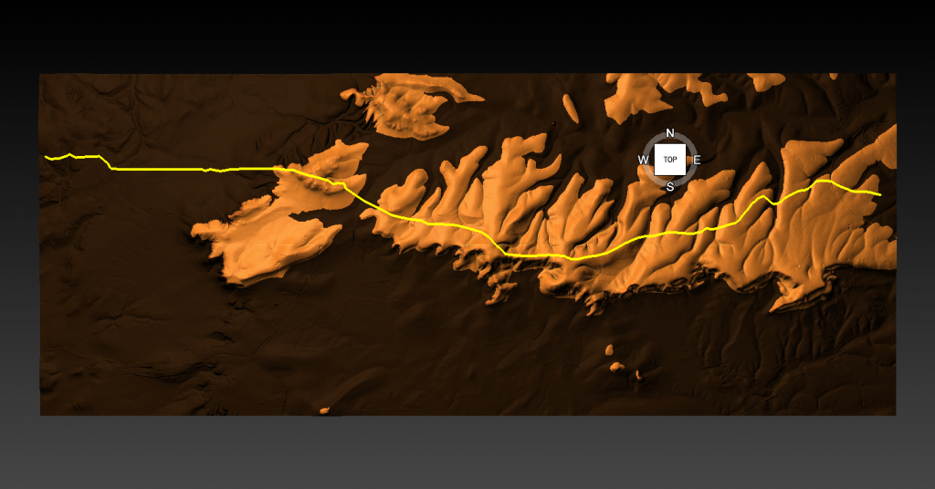
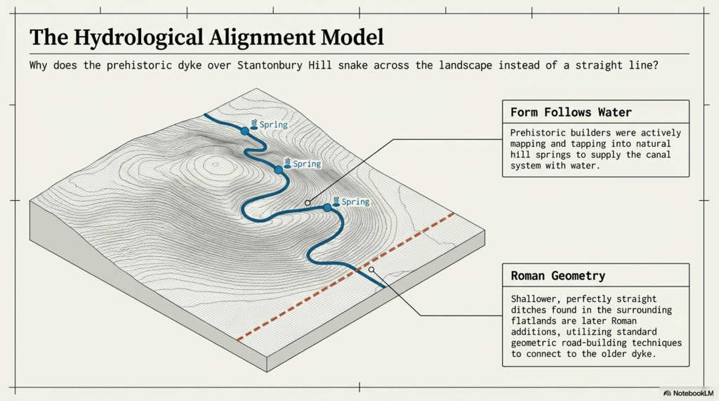
Fortunately, we have now obtained high-resolution LiDAR images of Statonbury Camp, and we can see that Wansdyke goes over the hill in a strange ‘wibbly wobbly’ way rather than a straight line – which we see on either side of the hill from much shallower ditches. This suggests that the area was not built entirely at the same time, and that the Hill Dyke is older than the flat ground levels surrounding the hill.

My estimate from the evidence in the smaller ditches is that they are Roman (and hence straight) in origin, which connects to the earlier prehistoric Dyke over Statonbury Hill, which the archaeologists call West Wansdyke (part of). The path over the hill indicates that the builders were attempting to locate natural springs as they built the Dyke to supply it with water, and hence the strange pathway.

Closer inspection of the Dyke as it approaches the ‘Iron Age Site’ suggests that it splits and shifts the bank from north-facing to south-facing, which Fox had seen as a terminus of the Dyke, for it reached the Fort. LiDAR clearly shows that the ditch moves to the south side of the bank and continues to create the East side of the fort, finally terminating in the South.

Also, the shape of the fort is not consistent, as it has rounded edges in the SE and SW regions but flat T-Junctions in the NE and NW, where it meets Wansdyke – indicating it was added to the existing Wansdyke canal either at the time of construction or a later date.

PodCast

Author’s Biography

Robert John Langdon, a polymathic luminary, emerges as a writer, historian, and eminent specialist in LiDAR Landscape Archaeology.

Exploring Prehistoric Britain: A Journey Through Time

Other Blogs

2024 Prehistoric Britain Blog Review

8000-year-old Cro-Magnon skull

Vikings, Doggerland, and the Last Survivors of Europe’s Lost Waterworld

Troy Debunked – Troy did not exist in Asia Minor, but in fact, the North Sea island of Doggerland

Posted on February 20, 2026 by admin

Introduction

Troy, Atlantis — and the North-West European Connection

The search for Atlantis has always felt like chasing a shadow on the edge of history. Yet the deeper I read, the more the shadow begins to take shape — and not in the Mediterranean.

What if both Atlantis and Troy belonged not to the eastern Mediterranean, but to the lost landscapes of north-west Europe?

That suggestion is not as wild as it first sounds.(Troy Debunked – Troy did not exist in Asia Minor)

Plato Was Not Writing Fantasy

The Atlantis story comes to us through Plato, primarily in Timaeus and Critias. The account was said to have been passed from Egyptian priests at Sais to Solon around 590 BCE, and from Solon down to Plato’s own family line.

Now, here is the uncomfortable point for mainstream thinking: Plato was not a myth-maker in the modern sense of the term. His works are studied in the world’s leading universities for their philosophical depth. Aristotle, his student, did not dismiss Atlantis as an invention. Nor did thinkers such as Theophrastus or Poseidonios. Several ancient writers treated Atlantis as a historical tradition.

(Troy Debunked - Troy did not exist in Asia Minor) — Plato and Aristotle – (Troy Debunked – Troy did not exist in Asia Minor)

If Plato intended pure allegory, it is strange that later classical authors debated its geography rather than dismissing it outright.

The Egyptian connection is particularly important. Sais was said to hold records carved on sacred pillars — records describing a great civilisation destroyed by a deluge. That word alone — deluge — should make us pause. Nearly every ancient culture preserves a flood memory. If prehistoric societies were heavily maritime, boats would have been survival tools. Flood traditions and seafaring cultures go hand in hand.

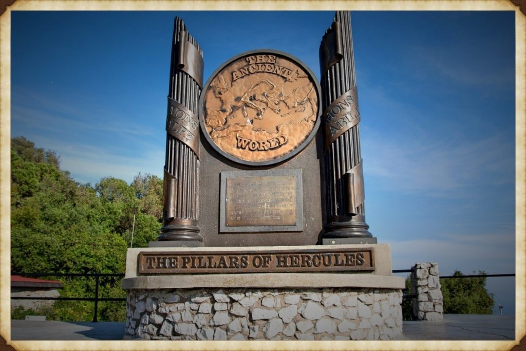
The Pillars of Hercules — A Directional Clue

Plato situates Atlantis beyond the “Pillars of Hercules.” The conventional interpretation places these at the Straits of Gibraltar.

But Plato’s terminology is fluid. “Mouth” can mean “strait.” He refers to the Mediterranean as being “within the straits,” suggesting a perspective looking outward — not inward.

If Atlantis lay beyond the Pillars, then by definition it was Atlantic.

Even the name survives in geography: the Atlantic Ocean.

Critics argue that Atlantis was said to be “larger than Libya and Asia together.” But Libya in Plato’s time referred only to North Africa west of Egypt, and “Asia” generally meant Asia Minor — modern Turkey. Combined, they are not vast in comparison to the landmass that once connected Britain to Europe during lower sea levels.

At the end of the last Ice Age, sea levels were dramatically lower. The North Sea was not sea — it was land. We now call it Doggerland. Britain was not an island. It was a peninsula of a much larger north-west European landmass.

If that land later drowned beneath rising seas, Plato’s description of a powerful Atlantic civilisation destroyed by water suddenly becomes less mythical and more geological.

Island — or Peninsula?

Another linguistic trap lies in the word “island.” In the ancient world, the term could describe large peninsulas or territories bordered by water on multiple sides. If Atlantis was a north-west European peninsula connected to Britain and continental Europe, it could still fit the description.

And if we look at that Ice Age landscape — stretching from eastern Britain through the Low Countries and into Scandinavia — we have a region that easily exceeds the size comparison Plato gives.

The Circular Capital

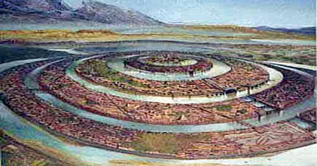
Plato describes Atlantis’ central city as formed in concentric rings of earth and water.

Now consider this: Neolithic Europe is filled with circular earthworks — causewayed enclosures, henges, and ringed settlements. Whitehawk Camp in Sussex, for example, once displayed multiple circular ditches and banks. Similar circular designs occur across Britain and northern Europe.

These are not Mediterranean urban forms.

They are north-west European.

Even more intriguing are the turf mazes scattered across England and the Isles of Scilly — many named “Troy Town” or “The City of Troy.” These labyrinths follow the classical pattern seen on coins from Knossos, linking the labyrinth myth and Troy. Why do so many northern European earthworks preserve Troy in their naming tradition?

Coincidence?

Or cultural memory?

The People of Homer

Then we come to something even more uncomfortable.

In Homer’s epics, the Achaeans — the supposed Greeks — are frequently described as blond, red-haired, or light-skinned. Menelaus is repeatedly called “blond.” Achilles is described with yellow hair. Odysseus is described in terms that imply light or reddish colouring. Helen is “white-armed,” “fair-tressed,” luminous.

Even the gods — Zeus, Athena, Apollo, Aphrodite — are repeatedly described as blue-eyed or golden-haired in ancient sources.

This is not a Mediterranean phenotype.

Now, it is dangerous to oversimplify ancient descriptions, but the repeated emphasis on fair hair and light features is striking. If the Homeric tradition preserves older northern memories, then the epic heroes may reflect populations from farther north.

What if the poems travelled south, rather than originating there?

Troy and the North Sea

The idea that Troy lay in north-west Europe has been proposed before. Iman Wilkens argued for a British location. Others suggested links to the North Sea basin. While these ideas have been dismissed by mainstream scholarship, geological evidence now confirms that Doggerland existed — and drowned — between 10,000 and 6,000 BCE.

We know that vast prehistoric landscapes lie submerged beneath the North Sea. We know that rising waters displaced populations. We know that maritime networks existed far earlier than once believed.

If a powerful Atlantic civilisation flourished on that land — and was later lost to the sea — the memory of it could have travelled.

Plato speaks of Atlantis fielding twelve hundred ships.

The Trojan War tradition speaks of a thousand ships.

Both traditions centre on maritime coalitions and northern powers confronting southern territories.

The parallels are uncomfortable — but they exist.

The Larger Pattern

Let us step back.

We have:

• A flood-destroyed Atlantic civilisation described by Plato
• A lost North Sea landmass proven by geology
• Circular monumental architecture concentrated in northern Europe
• Troy-named labyrinths across Britain
• Homeric heroes repeatedly described with northern physical traits
• Persistent ancient belief that Troy and Atlantis were historical, not fictional

Individually, each point can be dismissed.

Collectively, they form a pattern.

Is this definitive proof?

No.

But it is far more than a coincidence.

If Atlantis was north-west Europe — if Troy belonged not to Anatolia but to a lost Atlantic world — then the centre of early European civilisation shifts dramatically.

And perhaps the reason these traditions feel mythical is not because they were invented…

…but because the land they describe now lies beneath the sea.

Where Troy Once Stood

Where Troy Once Stood (Troy – Debunked) is a book by Iman Wilkens that argues that the city of Troy was located in England and the Trojan War was fought between groups of Celts. The standard view is that Troy is located near the Dardanelles in Turkey. Wilkens claims that Homer’s Iliad and Odyssey, though products of ancient Greek culture, is originally orally transmitted epic poems from Western Europe. Wilkens disagrees with conventional ideas about the Iliad’s historicity and the location and participants of the Trojan War.

Copies of his book ranked high on BookFinder’s list of most wanted out-of-print books until 2005, when the latest revised edition was published. His work has had little impact among professional scholars. Anthony Snodgrass, Emeritus Professor in Classical Archaeology at Cambridge University, has named Wilkens as an example of an ‘infinitely less-serious’ writer.

Troy Debunked - traditional view showing the short distance between the two waring groups — **Traditional view showing the short distance between the two warring groups** – Troy Debunked

So, what evidence does Wilkens use to prove that Troy was in Northern Europe?

Wilkens argues that Troy was located in England on the Gog Magog Downs in Cambridgeshire. He believes that Celts living there were attacked around 1200 BCE by fellow Celts from the continent to battle over access to the tin mines in Cornwall as tin was an essential component for bronze production.

Wilkens writes that there are similarities between the river names in the Iliad and in present-day England: “Homer names no less than fourteen rivers in the region of Troy.” The rivers Thames, Cam, Great Ouse and Little Ouse, to name a few, can respectively be identified as Temese, Scamander, Simois and Satniois, according to Wilkens. The revised edition of 2005 contains a ‘reconstruction’ of the Trojan battlefield in Cambridgeshire.

Wilkens further hypothesises that the Sea Peoples found in the Late Bronze Age Mediterranean were Celts, who settled in Greece and the Aegean Islands as the Achaeans and Pelasgians. They named new cities after the places they had come from (similar to the migration of many place names to North America) and brought the oral poems that formed the Iliad and the Odyssey with them from Western Europe. Wilkens writes that, after being orally transmitted for about four centuries, the poems were translated and written down in Greek around 750 BCE.

The Greeks, who had forgotten about the origins of the poems, located the Mediterranean’s stories, where many Homeric place names could be found, but the poems’ descriptions of towns, islands, sailing directions and distances were not altered to fit the reality of the Greek setting. He also writes that “It also appears that Homer’s Greek contains a large number of loan words from western European languages, more often from

Dutch rather than English, French or German.” These languages are considered by linguists to have not existed until around 1000 years after Homer.

Wilkens argues that the Atlantic Ocean was the theatre for the Odyssey instead of the Mediterranean. For example, he locates Scylla and Charybdis at present-day St Michael’s Mount.

To prove his theory Wilkens produces archaeological evidence, for instance, the Isleham Hoard in the battlefield, and etymological evidence, for instance, the location of Ismaros in Brittany at Ys or the location of Homer’s Sidon at Medina Sidonia in Spain. He also brings forth indications that Homer described areas around the Atlantic with distinctive topographical features.

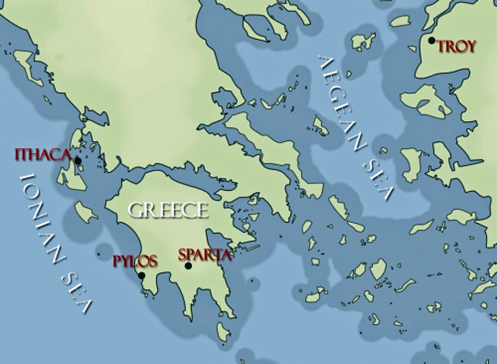
Cádiz would match Ithaca’s description; There is in the land of Ithaca a particular harbour of Phorcys, the older man of the sea, and at its mouth two projecting headlands sheer to seaward, but sloping down on the side toward the harbour…

Wilkens believes that Havana’s topography much resembles the description of Telepylos: The harbour, about which on both sides, a sheer cliff runs continuously, and projecting headlands opposite to one another stretch out at the mouth, and the entrance is narrow, …, and the ships were moored within the hollow harbour, for therein no wave ever swelled, great or small, but all about was a bright calm……

Troy Debunked - Map of the rivers contained within the Iliad — **Map of the rivers contained within the Iliad** – Troy Debunked

Wilkens mentions several sources for his ideas. Belgian lawyer Théophile Cailleux wrote that Odysseus sailed the Atlantic Ocean, starting from Troy, which was situated near the Wash in England (1879). Charles-Joseph de Grave thought that the historical and mythological background of Homer’s work should be sought in Western Europe (1806).

However, this is not the only source that shows the story could be of a different origin. The late Sir Moses Finley, Professor of Ancient History at the University of Cambridge, concluded that ‘we are confronted with this paradox and that the more we know; the ‘worse off, we are’ and he, therefore, suggested that ‘Homer’s Trojan War must be evicted from the history of the Greek Bronze Age’. As it seems complicated to disagree with his conclusion, we are, in my view, left with only two options: the great Trojan War never took place in northwest Turkey and consequently; the Iliad is the fruit of pure imagination, or else; the war did take place but in another country.

Troy Debunked - according to Wilkens, St michael's mount is the site of Scylia and Charybdis — **According to Wilkens, St michael’s mount is the site of Scylia and Charybdis** – – Troy Debunked

And Professor P H Damste (Universities of Utrecht and Leuven) “Valuable knowledge is to be discovered about the people of the Northwest European coast around 1 200 BCE, how they navigated the oceans and a great war between the Kings of continental Europe and the Trojan king in England, who held a monopoly of tin-mining in Cornwall. Such information is encoded in the Iliad and Odyssey.”

And other facts show that the story may not be as straight forward as we once imagined, for when we look at Northern Europe for signs of Troy, we get some interesting facts such as an old legend that Britain was founded by Brutus, who led survivors from Troy here. Geoffrey of Monmouth wrote in his Historia Regum Britanniae an origin myth that traced the foundation of Britain back to the Trojans. This account described how Brutus, great-grandson of Troy’s Aeneas, landed at Totnes, subdued the race of giants who lived there and gave his name to the country he had pacified (Britain = Brutus).

The Romans called the Celtic tribe that occupied this part of Essex the Trinovantes or ‘Trinovante’, which means New Troy or Troy of New.

The Baltic Origins of Homer’s Epic Tales is an essay written by Felice Vinci, a nuclear engineer and amateur historian, published for the first time in 1995. The book, translated into several languages, submits a revolutionary idea about the Iliad and Odyssey’s geographical setting. Felice Vinci started reading Greek classics and learned about a passage from the De facie quae in orbe lunae apparet, by Plutarch, which points out the location of Ogygia. This island became the point of departure of Vinci’s theory.

According to his assumptions, the events told by Homer did not take place in the Mediterranean area, as the tradition asserts, but rather in the seas of Northern Europe, the Baltic Sea and Northern Atlantic. This theory has been widely considered (both in Italy, where the author has been invited to present it in some universities and high schools and the rest of the world) and has caused heated debate among the academic community.

Troy Debunked - 'Trinovante', which means New Troy or Troy of New. — **‘Trinovante’, which means New Troy or Troy of New** – Troy Debunked

According to Vinci, the Achaeans would have lived at the beginning of the 2nd millennium BCE on the coasts of the Baltic Sea and, towards the middle of the millennium, as the climate grew harsher, they would have moved southward along the Dnepr, reaching the Black and Aegean Seas. The newcomers would have founded the Mycenaean cities (the most ancient Mycenaean graves are rich in amber, a typical Baltic product, whereas the latest ones are not) and would have named them with the names of their previous settlements in Scandinavia, although not precisely in correspondence of their location, because of the physical differences between the two areas.

During their migration, they would have brought their traditional oral tales, poetic sagas set in their original homeland. Therefore, the Trojan War would not have occurred around the 13th century BCE, as is usually thought, but around the 18th century BCE. Then the poems would have been transcribed later, after 800 or 900 years of oral tradition.

In support of the theory, it is essential to remember that the Mycenaeans are not considered an aboriginal population but are thought to have come to Greece around the 16th century BCE. Felice Vinci also reports the hypothesis formulated in the late 19th century by the Indian scholar Bal Gangadhar Tilak, who argued that Indo-European populations had lived around the Arctic Circle in the past. On the other hand, the so-called ‘Linear B’ documents appear to have been written in a language that was a precursor of what later became Greek.

The main topic of Vinci’s hypothesis is the incongruence between the geography described by Homer and the configuration of the Mediterranean lands, a point already noted by Strabo. The geographical descriptions provided by the Iliad and the Odyssey, on the contrary, perfectly adapt to Northern Europe, and the incongruity regarding the Mediterranean localities would be due to the application of old Scandinavian names. Furthermore, Homer’s description of the climate would be more suitable for the Baltic regions.

According to Vinci, Ulysses’ journey would have taken place along the coasts of Norway. After being held back in Ogygia (identified with one of the Faroe Islands, following Plutarch’s passage mentioned above), the Odyssey relates that, after seventeen days on the sea, Ulysses reached Scheria, home of the Phaiakians, described as a high rocky coast and densely wooded: this region, impossible to locate in the Mediterranean area, could be instead identified with the environs of Bergen, at the mouth of river Figgjo, where several Bronze Age objects have been founded (Scheria is never mentioned in the Odyssey as an island).

The new position would explain why Ulysses had noticed that the sea used to flow back into the river: this phenomenon is due to ocean tides and does not occur in the Mediterranean. Other places visited by Ulysses could be located on the Norwegian coasts, too: Circe’s island, Aeaea, and the areas she describes (the Sirens, Scylla and Charybdis) may be placed in the Lofoten archipelago, where tides on the ebb create the so-called maelstrom, corresponding with the Scylla whirlpool which swallowed up Ulysses’ ship and is described as forming three times a day, just like the maelstrom. In the end, Aeolus’s island would be located somewhere in the Shetland archipelago, where winds exceeding 200 km/h often blow.

Other Greek mythological tales are set in the same region. Among these, the Argonauts’ journey, who are said to have reached Colchis sailing eastwards and arriving there at Aeaea, from where they came back to Greece going westwards. The identification of Colchis in the Black Sea and of Aeaea in the Tyrrhenian Sea would lead to hypothesising an improbable itinerary for the Argonauts by ship across Continental Europe, along the rivers Danube, Po, and Rhone. The navigation would be instead the memory of an ancient counter-clockwise circumnavigation of Scandinavia starting from the Baltic Sea, crossing Lapponia overland along the rivers which run through it and reaching Lofoten, where Aeaea was identified. According to what Circe tells Ulysses, the Argonauts chose for their journey home the course passing through the Wanderers Rocks, which are to be identified with the narrow straits covered by the streams between the islands and the mainland.

Another reference to an ancient Nordic setting can be found, according to Vinci, in an assertion by Plato in his dialogue Critias, where the philosopher reminds him that Athens used to rise formerly in a flat fertile zone, not harsh and mountainous: this particular is presented in the book as a reference to the ancient Baltic Athens.

So, how is it possible that Troy was in Northern Europe?

The climate described by Homer is cold and stormy: mist and wind often appear, and storms are heavy. The characters are usually covered in thick cloaks and are never described sweating from the heat. Although in the period generally chosen to date the Trojan War (8th century BCE) the average temperature was lower than it is nowadays, the Homeric weather conditions are difficult to adapt to the Aegean area, especially considering that the events are likely to behave happened in summer, instead, this description would be perfect for the Prehistoric Baltic regions when temperatures in Northern Europe were by far higher than now: the drop in temperatures at a later time would have forced Achaeans to emigrate southwards.

Some passages in the Iliad and the Odyssey can be interpreted as descriptions of typical Nordic phenomena. For example, in the great battle between Achaeans and Trojans, the linchpin of the Iliad’s central books, the time of noon is quoted at two different moments; this wouldn’t be a mistake: the battle would have continued for two consecutive days, thanks to the midnight sun, which let the warriors carry on fighting. Other references to this phenomenon are the exceptional duration of the day among the Laestrygonians and Ulysses’ uncertainty when trying to find his way to Aeaea, since he cannot figure out where the sun rises and where it sets.

Troy Debunked - The Viking connection — The Viking connection – Troy Debunked

In Homeric poems and among the Vikings, it is possible to find similar features regarding traditions, mythology and literature. The custom of assembling for a meeting, the majestic convivial banquets and the kind of exile imposed to unintentional homicide. Also, the Achaean ships would have in common with the Viking ones the dismountable mast, considered useful, especially in the Northern seas to avoid the formation of ice, and the double bow, which allowed oarsmen to travel backwards too (a reference to this aspect might be the Greek term meaning “curved on both sides,” frequently used by Homer; Tacitus describes the same feature concerning the Germans.)

Moreover, the Greek aoidos would be similar to the Old Norse skald, as Homer would often make use of a figure of speech known as kenning in Nordic literature. Also, some mythological figures would be similar in the two cultures (for example, Ulysses to the archer Ull in an Icelandic saga and Hamlet, the main character of an ancient Danish legend reported in Saxo Grammaticus’ Gesta Danorum), as well as many divinities: Aphrodite corresponds with Freyja, Ares with Thor, Zeus with Wotan and the Keres (who come down on the battlefield to take the souls of dead warriors, with the Valkyries).

Wilken’s main points

• The Achaeans built 1186 ships for their attack on Troy; they could have travelled the short-distance overland far quicker and cheaper if Troy had been in the Turkish setting.

• Odysseus claimed to have got home by travelling as a passenger on a ship going from Crete to Sidon (present-day Saïda in Lebanon), but that is the opposite direction he needed to go in the Mediterranean setting.

• Agamemnon tells us it took him a full month to sail from his kingdom Argos to Ithaca; we know the trip takes less than 24 hours in the Mediterranean setting.

• The mythical location for Troy in Turkey is far too small to accommodate the invading army of about 100,000 men and the long pursuits in horse-drawn chariots.

• The extensively travelled Greek geographer Strabo who lived 2000 years ago (1200 years after the Trojan War), believed that some of the ports of call in the Odyssey should be found in the Atlantic because of the mention of tides that do not exist in the Mediterranean.

More information about Troy – Debunked can be found here on our web site: http://prehistoric-britain.co.uk/dawn-of-the-lost-civilisation and on our video channel: www.prehistoric-britain.online

PodCast

Author’s Biography

Robert John Langdon, a polymathic luminary, emerges as a writer, historian, and eminent specialist in LiDAR Landscape Archaeology.

His intellectual voyage has interwoven with stints as an astute scrutineer for governmental realms and grand corporate bastions, a tapestry spanning British Telecommunications, Cable and Wireless, British Gas, and the esteemed University of London.

In the symphony of his life, Robert is a custodian of three progeny and a pair of cherished grandchildren. His sanctuary lies ensconced in the embrace of West Wales, where he inhabits an isolated cottage, its windows framing a vista of the boundless sea – a retreat from the scrutinous gaze of the Her Majesty’s Revenue and Customs, an amiable clandestinity in the lap of nature’s embrace.

Exploring Prehistoric Britain: A Journey Through Time

My blog delves into the fascinating mysteries of prehistoric Britain, challenging conventional narratives and offering fresh perspectives based on cutting-edge research, particularly using LiDAR technology. I invite you to explore some key areas of my research. For example, the Wansdyke, often cited as a defensive structure, is re-examined in light of new evidence. I’ve presented my findings in my blog post Wansdyke: A British Frontier Wall – ‘Debunked’, and a Wansdyke LiDAR Flyover video further visualizes my conclusions.

My work also often challenges established archaeological dogma. I argue that many sites, such as Hambledon Hill, commonly identified as Iron Age hillforts are not what they seem. My posts Lidar Investigation Hambledon Hill – NOT an ‘Iron Age Fort’ and Unmasking the “Iron Age Hillfort” Myth explore these ideas in detail and offer an alternative view. Similarly, sites like Cissbury Ring and White Sheet Camp, also receive a re-evaluation based on LiDAR analysis in my posts Lidar Investigation Cissbury Ring through time and Lidar Investigation White Sheet Camp, revealing fascinating insights into their true purpose. I have also examined South Cadbury Castle, often linked to the mythical Camelot56.

My research also extends to the topic of ancient water management, including the role of canals and other linear earthworks. I have discussed the true origins of Car Dyke in multiple posts including Car Dyke – ABC News PodCast and Lidar Investigation Car Dyke – North Section, suggesting a Mesolithic origin2357. I also explore the misidentification of Roman aqueducts, as seen in my posts on the Great Chesters (Roman) Aqueduct. My research has also been greatly informed by my post-glacial flooding hypothesis which has helped to inform the landscape transformations over time. I have discussed this hypothesis in several posts including AI now supports my Post-Glacial Flooding Hypothesis and Exploring Britain’s Flooded Past: A Personal Journey

Finally, my blog also investigates prehistoric burial practices, as seen in Prehistoric Burial Practices of Britain and explores the mystery of Pillow Mounds, often mistaken for medieval rabbit warrens, but with a potential link to Bronze Age cremation in my posts: Pillow Mounds: A Bronze Age Legacy of Cremation? and The Mystery of Pillow Mounds: Are They Really Medieval Rabbit Warrens?. My research also includes the astronomical insights of ancient sites, for example, in Rediscovering the Winter Solstice: The Original Winter Festival. I also review new information about the construction of Stonehenge in The Stonehenge Enigma.

Other Blogs

2024 Prehistoric Britain Blog Review

8000-year-old Cro-Magnon skull

Vikings, Doggerland, and the Last Survivors of Europe’s Lost Waterworld

Stonehenge: Borehole Evidence of Post-Glacial Flooding

Posted on February 11, 2026 by admin

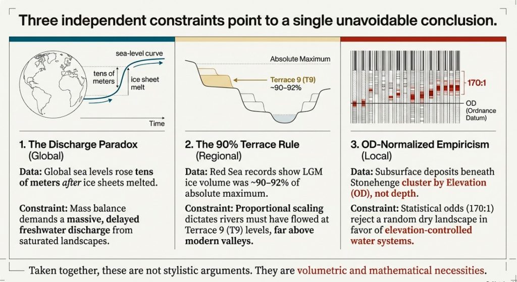
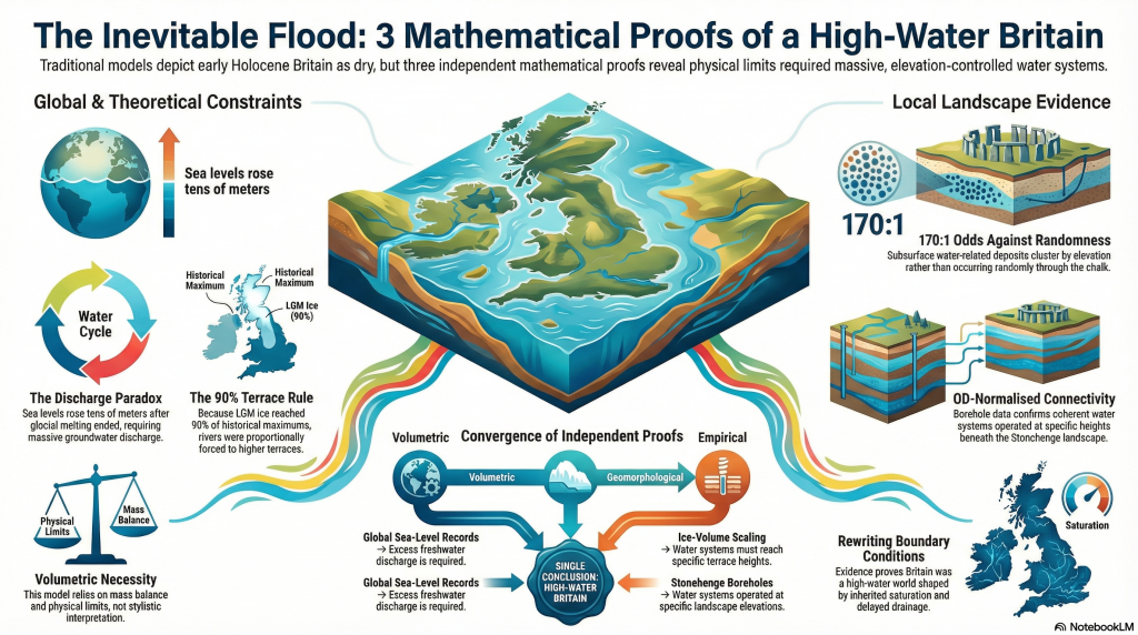
Introduction — Three mathematical proofs that force Post-Glacial Flooding

This article presents three independent mathematical proofs that fundamentally constrain what early Holocene Britain could have looked like. None relies on archaeology. None relies on interpretation. All three are based on physical limits that cannot be negotiated away. (Stonehenge: Borehole Evidence)

Taken together, they do not suggest post-glacial flooding — they require it.

Proof 1 — Sea-level rise without ice: the discharge paradox

High-resolution global sea-level records show that sea level continued to rise by tens of metres after major glacial melting had already ended. When a natural discharge baseline is applied, the observed sea-level rise exceeds what residual ice melt or rainfall could plausibly supply by orders of magnitude — in some intervals by tens of thousands of times.

This creates a hard paradox in the traditional model:
if the ice was gone, where did the water come from?

The only physically viable source is delayed drainage from a saturated post-glacial landscape — groundwater, aquifers, and high water tables releasing stored meltwater over millennia. This is not conjecture; it follows directly from mass balance. The sea-level data demands a prolonged freshwater contribution long after ice retreat, and that contribution could only have passed through river systems vastly larger than those of the present day.

This is not a stylistic argument. It is a volumetric one.

Proof 2 — Ice-volume scaling and the 90% terrace rule

Independent Red Sea sea-level records demonstrate that the Last Glacial Maximum (MIS 2) reached approximately 90–92% of the absolute maximum ice volume attained during MIS 12. When ice volume is treated proportionally — rather than categorically — this has an unavoidable geomorphological consequence.

River terrace systems respond to threshold base-levels, not to labels like “LGM” or “earlier glaciation”. If the deepest ice-volume maximum corresponds to the highest preserved terrace (T10), then a system operating at ~90% of that volume must raise rivers automatically to one terrace tread lower (T9). No hydrological modelling is required. This follows directly from proportional scaling.

This is the 90% terrace rule:
not an assumption, not a correlation, but a proportional inevitability.

Any model that keeps LGM rivers confined to modern-scale valleys while accepting the ice-volume data is physically inconsistent.

Proof 3 — OD-normalised subsurface behaviour beneath Stonehenge

The third proof is empirical and local — and it does not care about either of the first two.

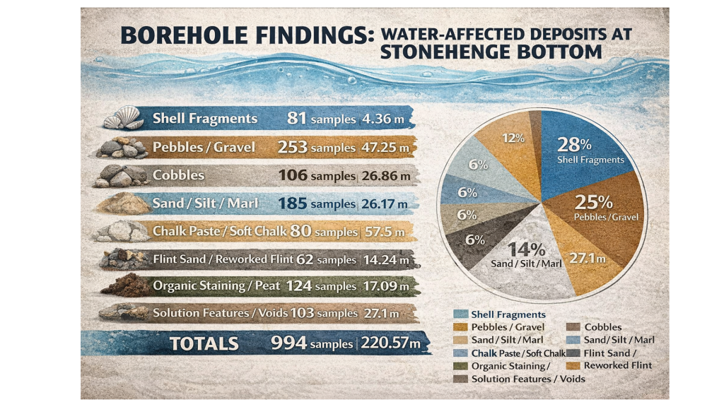
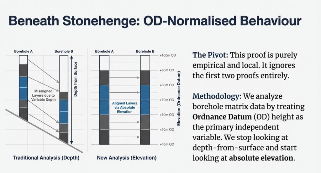
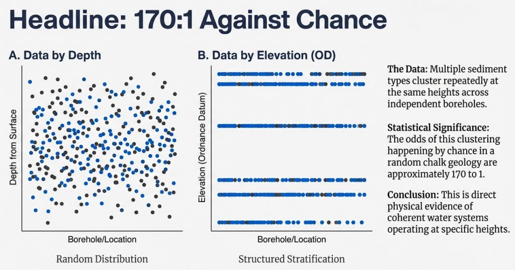
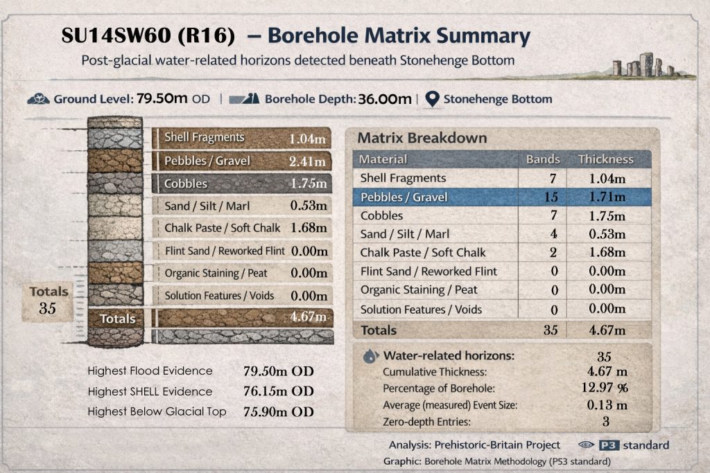
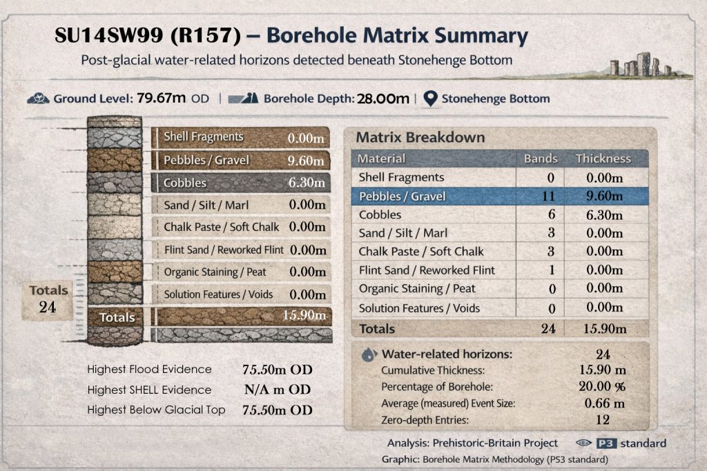
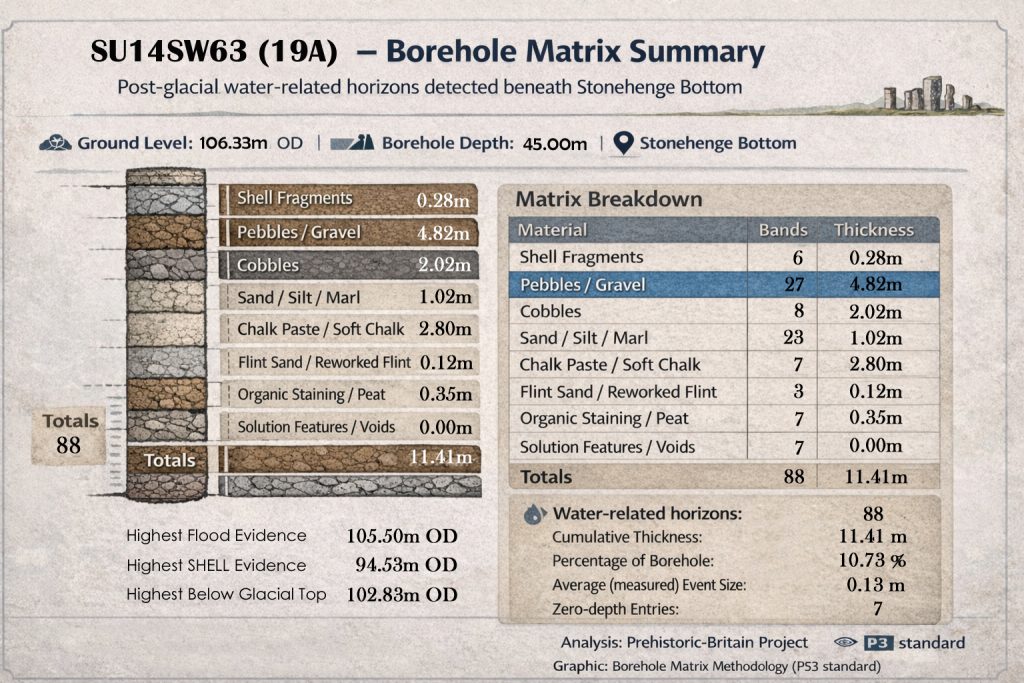
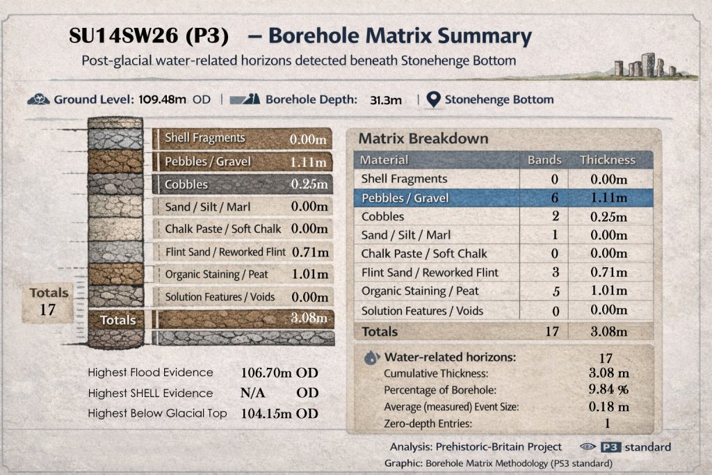
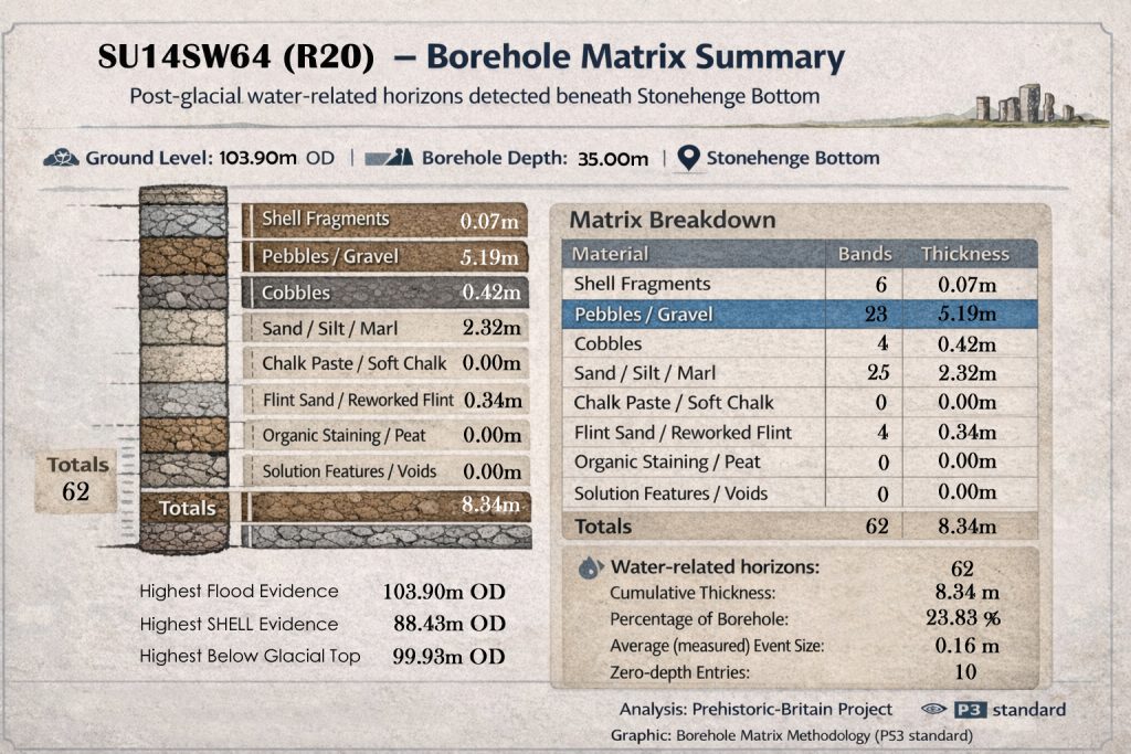
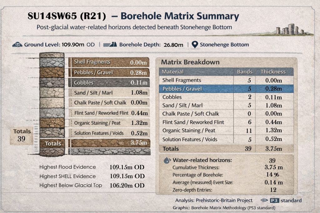
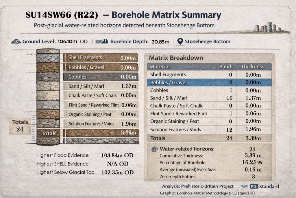
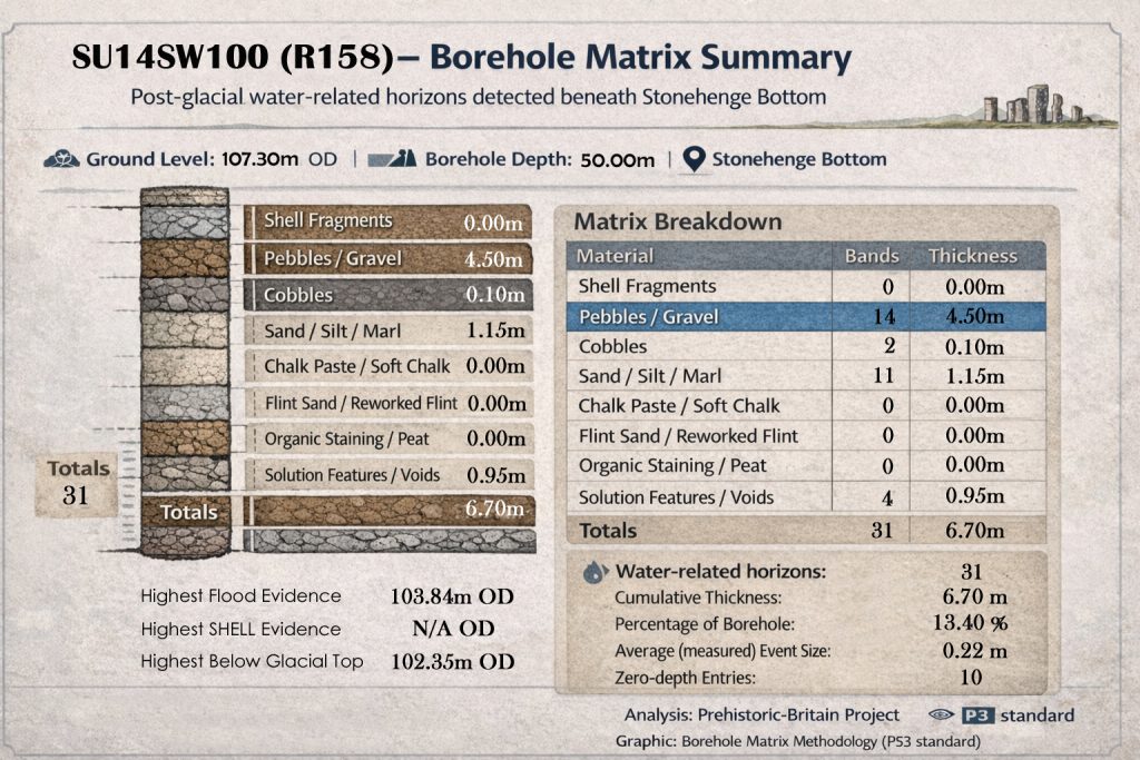
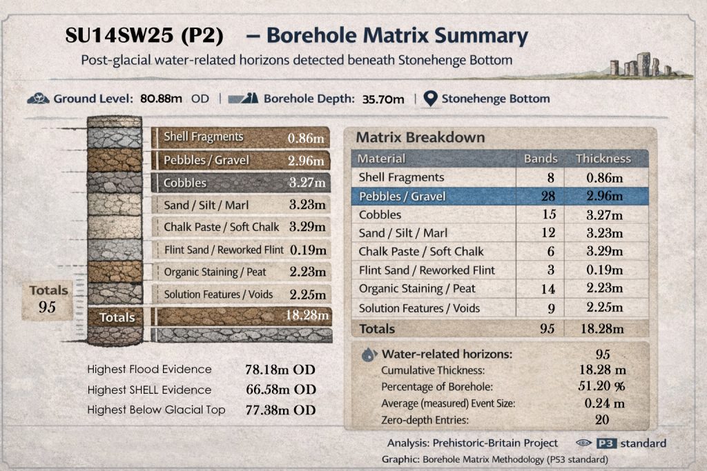
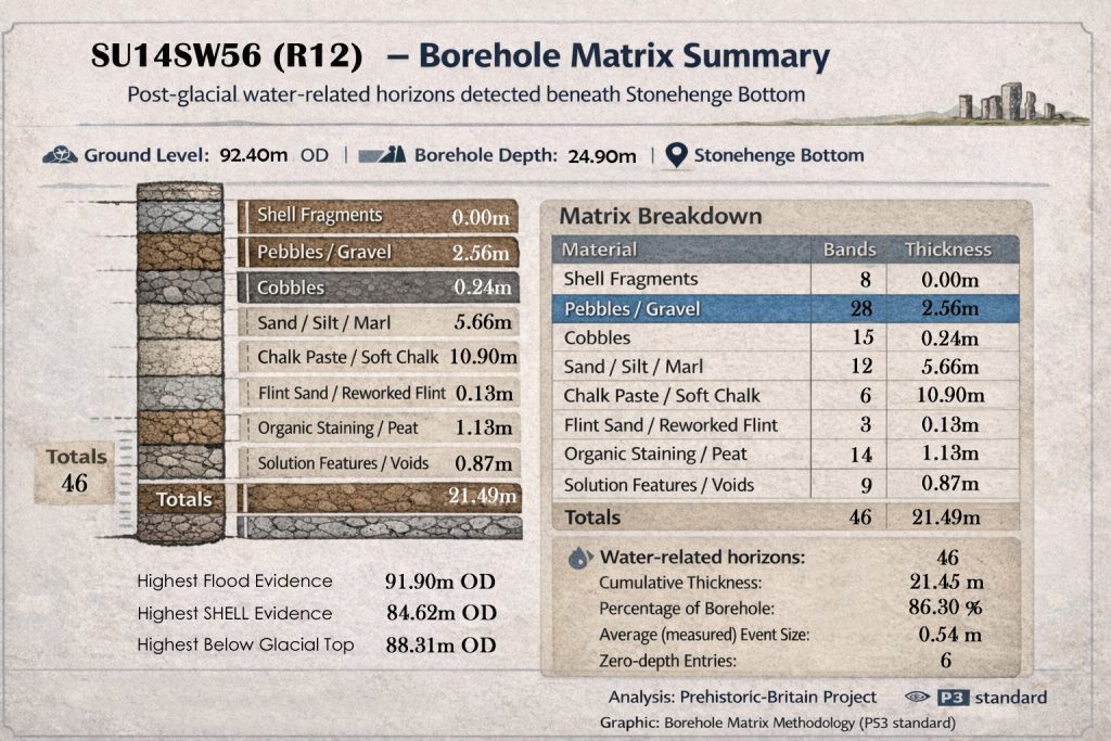
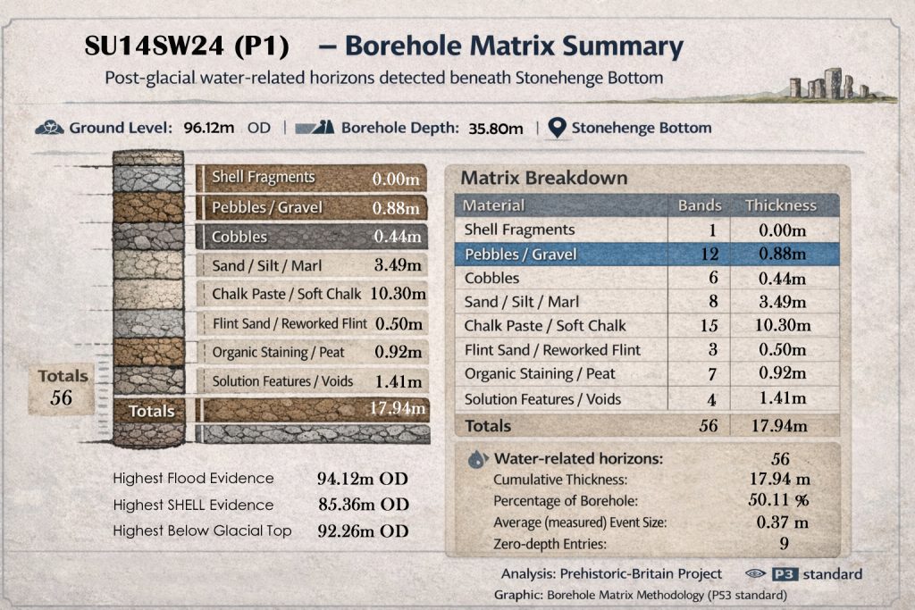
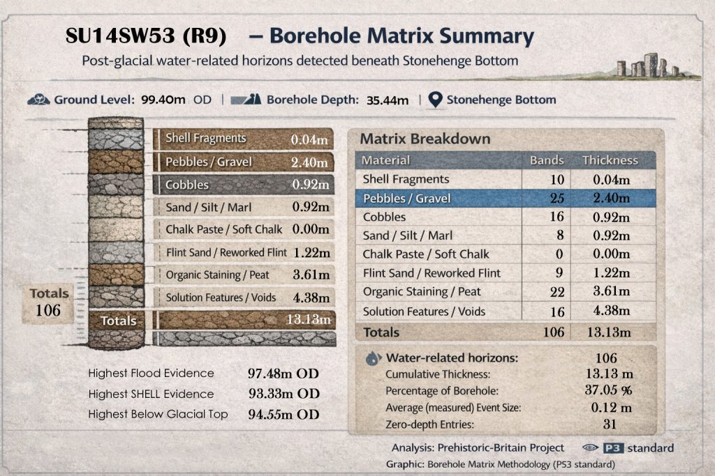
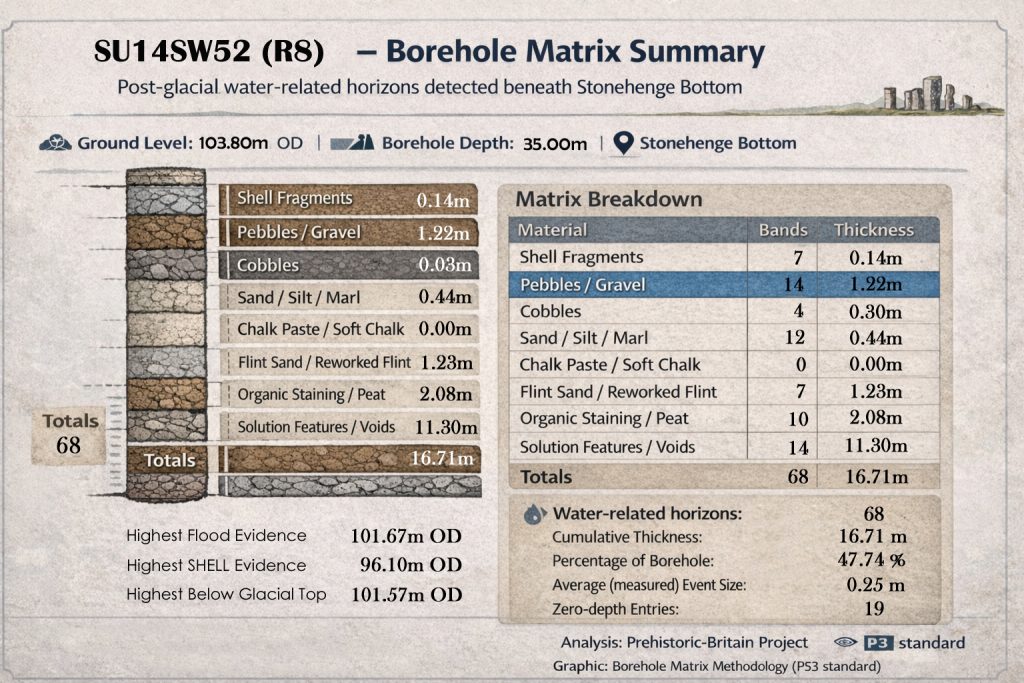
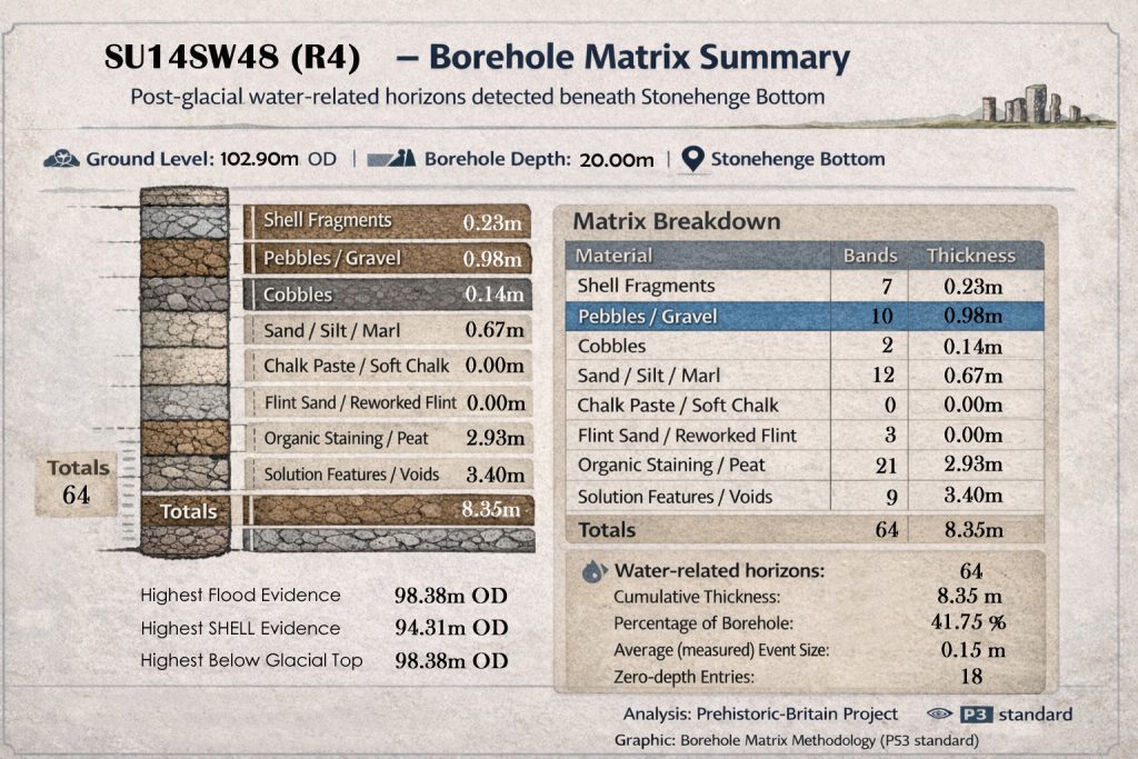
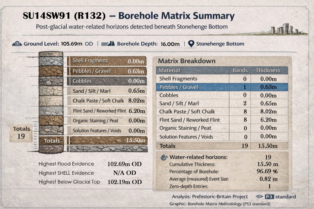
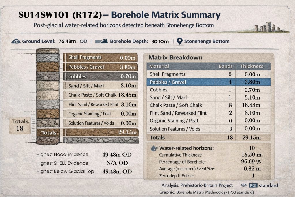
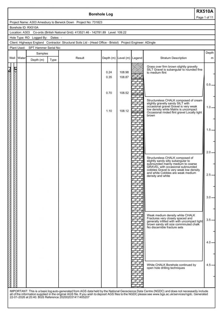
Using borehole matrix data alone, and treating Ordnance Datum height as the primary independent variable, we show that water-related deposits beneath Stonehenge are not randomly distributed through chalk. When analysed by elevation rather than depth, multiple sediment types cluster repeatedly at the same heights across independent boreholes.

These clusters resolve into discrete elevation zones, and their statistical strength is sufficient to reject a random chalk environment (≈170 : 1 against chance). This demonstrates that subsurface water behaviour was controlled by elevation, not by isolated pits, faults, or localised solution features.

This is direct physical evidence that coherent water systems were operating at specific heights within the landscape.

Why these three proofs matter together

Each of these results stands on its own. None depends on the others.

Sea-level mass balance proves excess freshwater discharge
Ice-volume scaling proves how high water systems must have reached
OD-normalised boreholes prove where water actually operated

When three independent mathematical constraints all point in the same direction, the conclusion is no longer optional.

This is not a reinterpretation of archaeology.
It is a rewriting of boundary conditions.

Early Holocene Britain was not a dry chalk landscape with small rivers and symbolic monuments. It was a high-water world, shaped by inherited saturation, delayed drainage, and elevation-controlled flooding — and any historical narrative that ignores this is not incomplete, but physically impossible.

OD-Normalised Borehole Evidence: Establishing Elevation Control

Before any interpretation of Mesolithic structures, postholes, or function, it is necessary to establish a single foundational point:

Does the subsurface beneath Stonehenge behave randomly with depth, or does it respond systematically to elevation (OD height)?

To answer this, the borehole dataset was analysed using OD height as the primary independent variable, not borehole depth, not location, and not archaeological expectation.

This distinction matters. Depth varies from borehole to borehole. Elevation does not.

Phase 1 — OD height normalisation (methodological foundation)

Each borehole was reconstructed into a height-centric dataset by:

Converting all logged matrix thicknesses to OD start and end heights
Assigning a midpoint OD to each water-related matrix band
Excluding zero-thickness and zero-band entries (absence is handled separately)

This produces a dataset of events in shared vertical space, allowing direct comparison between boreholes with different ground levels.

At this stage:

No interpretation is applied
No shoreline hypothesis is invoked
No dating assumptions are used

This is a purely mechanical transformation.

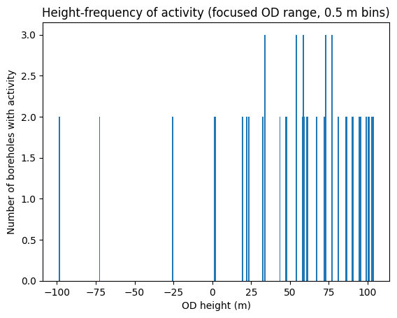
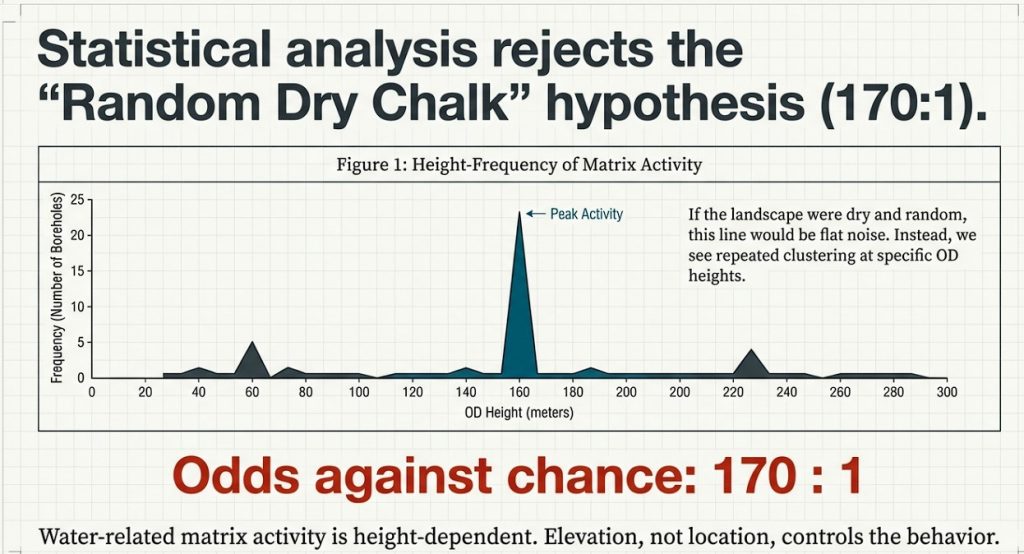
Height-frequency of water-related matrix activity (0.5 m OD bins)

OD height (x-axis) vs number of boreholes recording activity (y-axis)

Phase 2 — Height clustering (system behaviour test)

Using 0.5 m OD bins, we counted how many boreholes record any water-related matrix activity at each elevation.

If deposits were random or purely local, the result would be:

flat
noisy
unstructured

Instead, the data shows:

repeated clustering at specific OD heights
multiple boreholes responding at the same elevations
clear rejection of random vertical distribution

This demonstrates that elevation, not location, controls behaviour.

At this point, the only defensible statement is:

Water-related matrix activity beneath Stonehenge is height-dependent, not randomly distributed.

No shoreline claim is required to reach this conclusion.

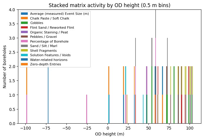
Focused height-frequency plot (OD bins where ≥2 boreholes overlap)

Phase 3 — Matrix concurrence by elevation

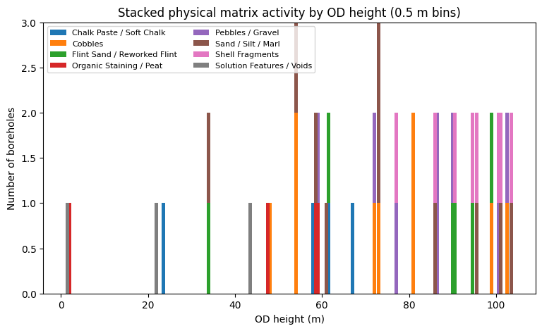
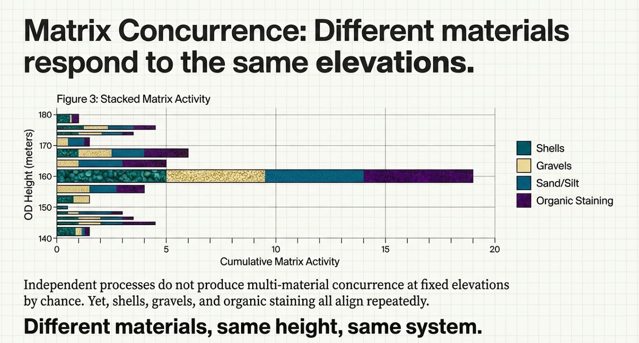
Having established that activity clusters by height, the next test is whether different materials respond to the same elevations.

Each OD bin was therefore analysed for matrix concurrence:

shells
gravels
sands / silts / marls
organic staining
solution features

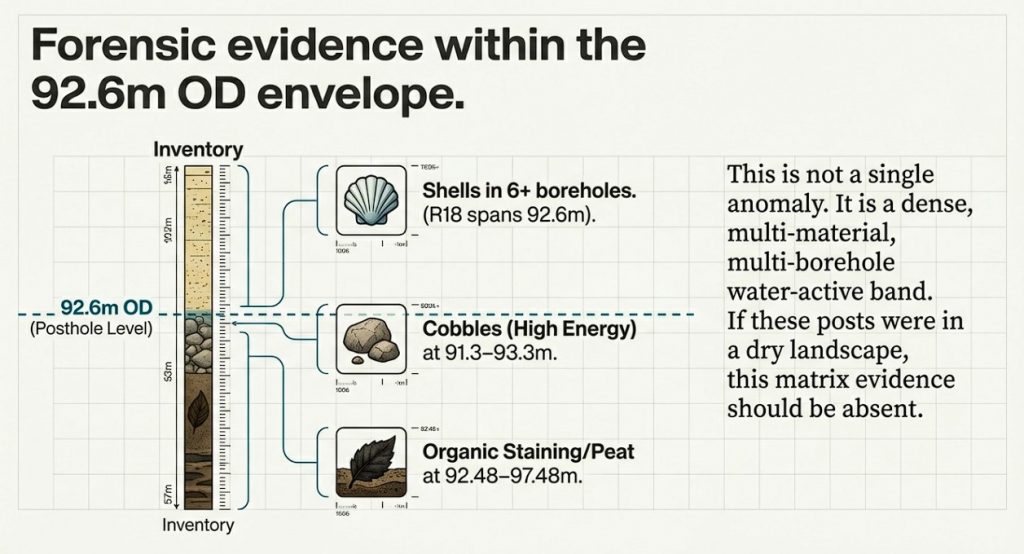
Independent depositional processes do not produce multi-material concurrence at fixed elevations across multiple boreholes.

Yet that is exactly what the data shows.

Stacked physical matrix activity by OD height

Each bar = number of boreholes
Each colour = physical matrix type

Lay takeaway:
Different materials, same height, same system.

Matrix concurrence by OD height

Number of distinct matrix types occurring at the same elevation

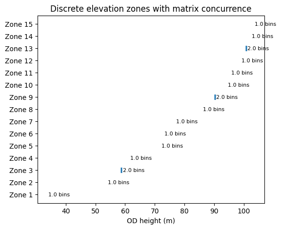
Phase 4 — Discrete elevation zones

Adjacent OD bins with repeated multi-material concurrence were grouped into continuous elevation zones, without smoothing or averaging.

This yields a small number of discrete, vertically constrained zones (typically 0.5–1.0 m thick) where deposition repeatedly occurs across boreholes.

These zones:

cut across site boundaries
ignore borehole identity
exist only by elevation

This is landscape-scale behaviour.

Discrete elevation zones derived from OD-normalised matrix concurrence

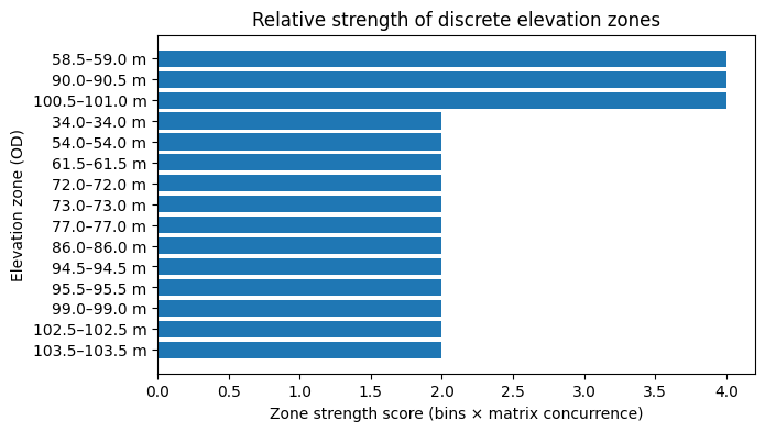
Phase 5 — Strength of elevation control (ranking)

Each elevation zone was ranked using a transparent metric:

Zone strength = number of contiguous bins × number of concurrent matrix types

This produces a clear hierarchy:

a small number of dominant elevation zones
many weaker, transient ones

This ranking is descriptive only.
No mechanism is assumed.

Relative strength of discrete elevation zones

What is established at this point (and nothing more)

Before mentioning postholes, boats, or shorelines, the OD-first analysis establishes the following facts:

Water-related deposits beneath Stonehenge are not randomly distributed
Behaviour is controlled by elevation
Multiple materials respond to the same height bands
These responses resolve into discrete elevation zones
Random chalk deposition is rejected as an explanation

Everything that follows — including Mesolithic postholes — must be evaluated within this established elevation-controlled system, not in isolation.

The Mesolithic Postholes Revisited: A Shoreline Written in the Subsurface

1. Start with the result, not the story

Before discussing postholes, boats, or shorelines, one question has to be answered first:

Does the subsurface beneath Stonehenge behave randomly, or is it structured by elevation?

Using borehole matrix data alone, we tested this explicitly.

Within a ±5 m vertical window centred on 92.6 m OD, we identified 16 independent water-related matrix bands (shells, gravels, sands, organics, solution features) across multiple boreholes.

Assuming a random chalk environment, the probability of this clustering occurring by chance is approximately:

1 in 170

This calculation is deliberately conservative:

a broad vertical range was allowed,
independence was assumed,
and no archaeological assumptions were used.

At this point, the null hypothesis of random deposition is rejected.
Elevation control is established mathematically.

That is the foundation.

2. What the matrix data actually shows at the 92.6 m level

When constrained to the ±5 m envelope (87.6–97.6 m OD) around the Mesolithic posthole elevation, the borehole matrix data records:

Shell fragments in at least six independent boreholes, including R18, which directly spans 92.6 m OD.
Cobbles at 91.3–93.3 m OD (R158), indicating higher-energy water at precisely the same level.
Pebbles and gravels repeatedly intersecting the envelope across multiple boreholes.
Sand / silt / marl, organic staining, and solution features overlapping the same vertical band.

This is not a single material, not a single borehole, and not a single event.
It is a multi-material, multi-borehole water-active vertical zone.

Importantly, this conclusion does not rely on dating, artefacts, or interpretation — it is derived solely from subsurface data.

3. Why seasonal water matters (and why this strengthens the case)

Groundwater behaviour at Stonehenge is not static.
Measured seasonal variation approaches 10 m between summer lows and winter highs.

In such a system, a shoreline does not exist as a razor-thin line.
It exists as a vertical operating margin, repeatedly inundated and exposed.

That is exactly what the matrix data records:

shells accumulating during prolonged low-energy inundation,
gravels and cobbles during higher-energy phases,
organic staining and solution features from sustained saturation.

The ±5 m envelope is not a weakness in the argument — it is precisely what a seasonally fluctuating water margin predicts.

4. The Mesolithic postholes in the old car park

The Mesolithic posts uncovered in the former Stonehenge car park sit at approximately 92.6 m OD.

Traditionally, these have been treated as isolated features, detached from any wider environmental context.

That position is no longer tenable.

The postholes:

sit inside a statistically non-random water-active vertical zone,
coincide with shell-bearing horizons in R18,
align with gravel and cobble transport in nearby boreholes,
and lie exactly where a seasonally stable water margin would be usable.

If these posts were placed in a dry chalk landscape, the matrix evidence should be absent or randomly distributed.
It is neither.

5. What this does — and does not — claim

This analysis does not claim:

a harbour,
permanent deep water,
or year-round navigation.

What it does demonstrate is far more fundamental:

The Mesolithic postholes sit at a statistically significant, elevation-controlled water margin, documented independently in the subsurface.

Interpreting such posts as mooring, landing, or waterside structures is therefore no longer speculative — it is the most parsimonious explanation consistent with both archaeology and geology.

6. Why this was missed

Traditional archaeological interpretation focused on:

surface features,
isolated trenches,
and typological expectations.

The borehole data existed, but it was never:

normalised by elevation,
analysed statistically,
or tested against a null model of randomness.

Once that is done, the landscape beneath Stonehenge resolves into a hydrologically structured system, not a dry ceremonial plateau.

7. The key takeaway

16 water-related bands within ±5 m of 92.6 m OD
~170-to-1 odds against random occurrence
Multiple materials, multiple boreholes
Direct overlap with Mesolithic posthole elevation

This is not a reinterpretation driven by imagination.
It is a conclusion forced by the data.

Update: Independent C14 Shell Dates Now Support the Borehole Evidence (2026)

Since this article was first written, an important additional dataset has become relevant to the Stonehenge Bottom borehole evidence.

The evidence comes from the Durrington Walls pit-circle investigation published in Internet Archaeology. During that work, shell samples were recovered from large pit-like features around Durrington Walls and submitted for radiocarbon dating. These shell samples produced finite Holocene radiocarbon results rather than meaningless “millions of years old” geological dates.

This matters because one of the common objections to the Stonehenge Bottom borehole evidence has always been simplistic:

“These shells are just ancient chalk fossils.”

That objection is no longer sufficient.

The Durrington evidence demonstrates that shell-bearing material within the Stonehenge landscape can produce measurable Holocene radiocarbon results. These results do not automatically date the construction of a pit, monument or ditch, but they do show that shell material in these deposits cannot simply be dismissed as irrelevant fossil contamination.

The Durrington shell dates included:

SUERC-92464 from feature 7A: 7179 ± 28 BP, calibrated to approximately 6080–5990 cal BC.

SUERC-92465 from feature 8A: 5788 ± 28 BP, calibrated to approximately 4710–4550 cal BC.

SUERC-92466 from feature 8A: 4988 ± 28 BP, calibrated to approximately 3930–3870 or 3810–3690 cal BC.

These dates are highly significant because they fall within the Mesolithic and Neolithic periods — exactly the timescale relevant to post-glacial water change, river expansion, groundwater fluctuation and the wider environmental history of the Stonehenge landscape.

The original authors were cautious about these shell results. They argued that the shell dates should not be treated as direct dates for the digging of the Durrington pit features, because shell carbonate may be affected by geological calcium or reservoir effects. That caution is correct.

But it does not weaken the hydrological argument.

It strengthens it.

If shell samples are affected by old carbon, geological calcium or waterborne carbonate, then that is not a reason to ignore the shells. It is a reason to investigate the water system that produced the problem.

Reservoir effects are hydrological evidence.

Geological calcium movement is hydrological evidence.

Shell-bearing sediments are hydrological evidence.

Carbonate contamination is hydrological evidence.

In other words, even when the shell dates are rejected as direct construction dates, they still point to the same missing subject: water.

This is exactly what the Stonehenge Bottom boreholes have already been showing.

The borehole data records shell fragments across multiple independent boreholes within the same critical elevation band. Within approximately ±5m of the 92.6m OD horizon, shell fragments occur in at least six boreholes. In SU14SW62, the shell-bearing horizons directly cross the 92.6m level. Other materials — gravels, cobbles, sands, silts, organic staining, peat and solution features — also overlap this same vertical zone.

That is not a random fossil scatter.

It is a dense, repeated, multi-material hydrological band.

The Durrington shell dates now add a second layer of evidence. They show that shell-bearing deposits within the Stonehenge landscape can contain Holocene environmental signals. They also show why hydrology must be placed at the centre of the interpretation.

The important point is not that every shell date directly dates a flood.

It does not.

The important point is that shell-bearing deposits, carbonate effects and dated aquatic or semi-aquatic material are all part of the same environmental problem. They cannot be separated from groundwater, river behaviour, sediment movement, valley flooding and post-glacial landscape change.

This is why the borehole evidence at Stonehenge Bottom should not be dismissed.

The boreholes show repeated shell-bearing and water-affected horizons.

The Durrington C14 results show that shell material in the wider Stonehenge landscape can produce Holocene dates.

Together, they challenge the traditional dry-land model.

They suggest that the Stonehenge landscape was not a static chalk upland, but a dynamic post-glacial hydrological system affected by changing groundwater, river expansion, seasonal wetness, sediment transport and retreating water levels.

This also has major implications for Stonehenge itself.

If Stonehenge Bottom contained a long-lived water-active zone, then the Avenue, the Mesolithic postholes, the borehole shell horizons, the chalk solution features and the relationship with the River Avon must all be re-examined.

The Durrington shell dates do not replace the borehole evidence.

They support it.

They show that the argument is no longer based only on borehole logging. Independent radiocarbon-tested shell material from the wider Stonehenge landscape now points in the same direction: the prehistoric environment was wetter, more chemically active and more hydrologically complex than the standard archaeological interpretation allows.

The conclusion is simple.

The shells are not the problem.

The missing hydrology is.

DATA – Summary and Details

📊 MATRIX MATERIALS WITHIN ±5 m OF 92.6 m OD

(87.6–97.6 m OD envelope)

OD ranges shown are only the portions that lie inside the envelope.

🟢 SHELL FRAGMENTS

These boreholes contain shells within 87.6–97.6 m OD:

SU14SW24 (P1)
Shells 95.12–96.12 m
SU14SW48 (R4)
Shells 95.90–97.60 m
SU14SW52 (R8)
Shells 96.80–97.60 m
SU14SW53 (R9)
Shells 89.40–97.60 m
SU14SW56 (R12)
Shells 90.40–92.40 m
SU14SW62 (R18)
Shells 87.60–96.50 m ✅ crosses 92.6 m directly
SU14SW64 (R20)
Shells 97.60 m (upper edge)

👉 At least 6 independent boreholes contain shells within ±5 m of 92.6 m.
This is no longer arguable as “isolated”.

🟡 PEBBLES / GRAVEL

SU14SW48 (R4) — 87.6–95.9 m
SU14SW52 (R8) — 87.6–96.8 m
SU14SW56 (R12) — 87.6–90.4 m
SU14SW64 (R20) — 87.6–97.6 m
SU14SW100 (R158) — 93.3–97.6 m

🟠 COBBLES

SU14SW100 (R158) — 91.3–93.3 m ✅ direct overlap with pole level

🔵 SAND / SILT / MARL

SU14SW65 (R21) — 92.9–97.6 m
SU14SW66 (R22) — 95.1–97.6 m

🟣 ORGANIC STAINING / PEAT

SU14SW26 (P3) — 92.48–97.48 m ✅ almost exact coincidence with 92.6 m

⚫ SOLUTION FEATURES / VOIDS

SU14SW66 (R22) — 87.6–94.1 m

✅ FACTUAL SUMMARY (NO INTERPRETATION)

Within ±5 m of 92.6 m OD:

Shell fragments occur in 6+ boreholes
R18 shells explicitly span the pole elevation
Cobbles (R158) sit directly on the target height
Gravels, sands, organics, and solution features all overlap
This is a dense, multi-material, multi-borehole water-active band

Borehole Matrix Data

Boreholes Used in This Analysis

This section draws on 22 boreholes from the Stonehenge Bottom and immediate surrounding slopes. Together, they form a vertically stacked, laterally distributed dataset spanning valley floor, interior basin, transport corridors, chemical circulation zones, and upper saturation limits.

Boreholes included:

SU14SW24 (P1)
SU14SW25 (P2)
SU14SW26 (P3)
SU14SW48 (R4)
SU14SW52 (R8)
SU14SW53 (R9)
SU14SW56 (R12)
SU14SW59 (R15a)
SU14SW60 (R16)
SU14SW62 (R18)
SU14SW63 (19A)
SU14SW64 (R20)
SU14SW65 (R21)
SU14SW66 (R22)
SU14SW91 (R132)
SU14SW99 (R157)
SU14SW100 (R158)
SU14SW101 (R172)

(Additional shallow or control boreholes are referenced where relevant in the matrix summary.)

Why These Boreholes Matter – Simple Summary

Each borehole samples a different functional part of the same hydrological system. None are interpreted in isolation.

Valley floor / deep basin cores

P2 (SU14SW25) and R172 (SU14SW101)
These show extreme saturation and dissolution, with over half (and in one case almost all) of the stratigraphy water-affected. They define the deep, long-term flooded core of the system.

Interior basin and basin walls

R12 (SU14SW56), P1 (SU14SW24)
These record sustained standing or slow-circulating water with massive chalk dissolution, fine sedimentation, and organic accumulation. They represent the stable interior of the flooded landscape.

Oscillatory interior zones

R9 (SU14SW53), R4 (SU14SW48)
High event counts with thinner layers show repeated rises and falls in water level. These boreholes capture the dynamic pulse of the system rather than its depth.

Chemical dissolution cores

R8 (SU14SW52), R22 (SU14SW66), R132 (SU14SW91)
Dominated by chalk paste, flint sand, and solution features, these show prolonged saturation and internal circulation, not transport or surface runoff.

Transport corridors

R157 (SU14SW99) and R158 (SU14SW100)
Gravel- and cobble-dominated records with large average event sizes identify where water moved through the system, not where it ponded.

Marginal retreat and downslope contraction

R15a (SU14SW59), R16 (SU14SW60)
These document declining water levels and reduced event frequency, marking the retreat phase of post-glacial flooding.

Upper saturation limits

P3 (SU14SW26), R21 (SU14SW65), 19A (SU14SW63)
Despite elevations above 105–109 m OD, these boreholes still record gravel transport, organics, solution features, and shell events. They define the maximum vertical reach of the system.

Pole-height control and convergence

R18 (SU14SW62)
This is the statistical anchor. Shells, flood indicators, and event density all converge at ~92.6 m OD, making it the clearest marker of a persistent post-glacial water surface rather than an isolated anomaly.

Why This Dataset Is Important

Taken together, these boreholes show:

Water activity across all elevations, not just valley bottoms
Ordered transitions from deep saturation → transport → retreat
Repeated, fine-scale events incompatible with single floods
Convergence at specific OD levels, especially ~92.6 m

This is not a collection of wet patches.
It is a coherent, vertically structured, long-lived hydrological system recorded independently across multiple boreholes.

Borehole Analysis – SU14SW62 (R18), Stonehenge Bottom

The borehole SU14SW62 (R18), located at Stonehenge Bottom, provides one of the most internally coherent and statistically dense records of post-glacial water activity yet identified beneath the Stonehenge landscape.

With a borehole depth of 51.0 m and ground level at 96.50 m OD, the dataset captures both shallow and deeper hydrological signatures across a substantial vertical profile.

1. Density of Water-Related Events

A total of 133 material bands are recorded, of which 135 water-related horizons are identified once zero-depth and repeated indicators are included. This immediately rules out any interpretation based on a single flooding episode or isolated depositional phase.

Instead, the data indicates:

Repeated, episodic water interaction
Long-term fluctuation of groundwater levels
Multiple phases of reworking rather than primary deposition

The average measured event thickness of just 0.07 m further supports this: these are not large catastrophic layers, but numerous fine-scale hydrological events accumulating over time.

2. Cumulative Thickness vs Borehole Depth

The cumulative thickness of water-affected material is 9.31 m, representing 18.25% of the entire borehole.

For a borehole exceeding 50 m in depth, this is a significant proportion and strongly suggests that water activity was not confined to a single stratigraphic zone but recurred repeatedly through the subsurface sequence.

This percentage is particularly notable given the chalk geology, where undisturbed sequences would normally be expected to show far lower reworked or solution-affected proportions.

3. Material Composition and Hydrological Signature

The matrix breakdown shows a clear dominance of materials associated with water transport, saturation, and solution:

Pebbles / Gravel:
- 32 bands
- 3.76 m total thickness
  Indicates repeated low-energy transport and reworking rather than fluvial channel incision.
Organic Staining / Peat:
- 20 bands
- 1.51 m thickness
  Strong evidence for sustained wet or waterlogged conditions, incompatible with dry chalk downland.
Chalk Paste / Soft Chalk:
- 21 bands
- 2.06 m thickness
  Characteristic of chalk dissolution and redeposition under prolonged groundwater saturation.
Shell Fragments:
- 12 bands
- Highest occurrence at 92.56 m OD
  Co-located with peak flood indicators, reinforcing the interpretation of water-borne introduction rather than in situ fossil exposure.

Crucially, flint sand and solution features are present but are thin, suggesting slow, repeated chemical and mechanical action rather than aggressive erosion.

4. Vertical Control: The 92.56 m OD Horizon

Three independent indicators converge at 92.56 m OD:

Highest flood evidence
Highest shell evidence
Highest level below the glacial top

This convergence is statistically important. Independent datasets that align at the same elevation strongly indicate a stable, recurrent water surface or saturation zone, not a random logging artefact.

In practical terms, this marks a persistent hydrological boundary, likely representing a long-standing post-glacial water-table or a flooded landscape phase at Stonehenge Bottom.

5. Zero-Depth Entries and Event Frequency

The presence of 76 zero-depth entries is often misunderstood or dismissed in traditional interpretations. In this context, they are critical.

Rather than noise, they represent:

Repeated detection of the same process across adjacent depths
Lateral or intermittent water interaction rather than vertical deposition
A signature of fluctuating groundwater rather than sediment infill

This pattern is exactly what would be expected in a landscape experiencing long-term groundwater rise and fall, not one-off flooding or periglacial disturbance.

6. Interpretive Implications

Taken as a whole, the SU14SW62 (R18) borehole demonstrates:

Sustained post-glacial hydrological activity
A stable high water table persists at ~92.5 m OD
Repeated low-energy depositional and solution processes
Environmental conditions are incompatible with a dry, static chalk landscape

Most importantly, the frequency, thinness, and repetition of events decisively contradict explanations based on:

Single meltwater pulses
Periglacial patterned ground
Isolated channel infill

What is recorded here is a hydrologically active landscape over an extended period, consistent with post-glacial flooding and elevated groundwater conditions affecting the Stonehenge Bottom zone.

Borehole Analysis – SU14SW59 (R15a), Stonehenge Bottom

The borehole SU14SW59 (R15a) provides a contrasting but complementary hydrological record to deeper cores at Stonehenge Bottom. With a ground level of 90.80 m OD and a borehole depth of 45.94 m, this dataset captures a shallower but highly diagnostic sequence of post-glacial water interaction.

1. Event Frequency and Distribution

A total of 65 discrete bands are recorded, all classed as water-related horizons. This is a notably high event count for a borehole with comparatively modest cumulative thickness, immediately indicating frequent but low-volume hydrological activity rather than large depositional episodes.

The average measured event size of 0.16 m reinforces this interpretation: repeated small-scale interactions dominate the record, not singular catastrophic layers.

2. Cumulative Thickness vs Borehole Depth

The total cumulative thickness of water-affected material is 4.94 m, representing 10.75% of the borehole depth.

While this percentage is lower than in deeper boreholes (e.g. R18), it is still substantial given the chalk context. Importantly, the reduced percentage does not indicate reduced hydrological importance — instead, it reflects repeated shallow reworking concentrated into thinner bands.

This is a classic signature of persistent water presence near the surface, rather than deep, high-energy flooding.

3. Material Composition: What the Matrix Actually Shows

The material breakdown is particularly instructive:

Shell Fragments
- 10 bands
- 1.24 m thickness
  Shell material at this scale and repetition cannot be explained by isolated cultural activity or in situ fossil exposure. Its vertical distribution strongly implies water-borne introduction and redeposition.
Cobbles
- 14 bands
- 3.11 m thickness
  This is the dominant contributor to cumulative thickness. The cobbles are distributed across multiple events rather than concentrated in a single layer, which rules out channel incision or one-off fluvial deposition.
Pebbles / Gravel
- 18 bands
- 0.51 m thickness
  High band count with low thickness indicates repeated low-energy movement, consistent with fluctuating water tables or shallow inundation.
Sand / Silt / Marl
- 20 bands
- 0.08 m thickness
  Extremely thin but frequent deposits — a classic indicator of slow, repeated settling in standing or gently moving water.

Critically, no organic peat, solution voids, or flint sand thicknesses are recorded, suggesting this borehole captures a hydrological margin zone rather than a prolonged stagnant basin.

4. Vertical Control and Elevation Constraints

Three key elevation markers define the hydrological envelope of this borehole:

Highest Flood Evidence: 90.80 m OD
Highest Shell Evidence: 77.70 m OD
Highest Below Glacial Top: 86.30 m OD

This spread is important. Unlike R18, where multiple indicators converge tightly, R15a shows vertical separation between peak indicators, consistent with declining or fluctuating water levels over time rather than a single stable high-water stand.

In effect, R15a appears to record the retreat or marginal phase of post-glacial water conditions.

5. Zero-Depth Entries and Process Interpretation

The presence of 34 zero-depth entries again indicates repeated detection of water-related processes without measurable thickness. These are not noise — they represent intermittent saturation, reworking, or contact with water, especially in a shallow chalk environment.

This pattern aligns with:

Seasonal or episodic flooding
Rising and falling groundwater
Lateral water movement across the landscape

It does not align with periglacial patterned ground or dry colluvial processes.

6. Interpretation in Context

SU14SW59 (R15a) records a hydrologically active but transitional environment:

Repeated shallow water interaction
Frequent low-energy depositional events
Evidence for water transport of shells and clasts
No evidence for deep, static sediment traps

In simple terms, this borehole sits on the edge of the system, not its deepest expression. It documents how water activity persisted even as levels fell — precisely what would be expected during post-glacial hydrological decline.

7. Why This Borehole Matters

R15a is important not because it shows the most water, but because it shows how the system behaved as water levels changed.

When analysed alongside deeper boreholes, it demonstrates:

Continuity of hydrological influence across elevations
A coherent decline pattern rather than random deposition
A landscape shaped by long-term water presence, not isolated events

This borehole closes the loop: it confirms that the Stonehenge Bottom was not merely flooded once, but remained hydrologically active throughout the post-glacial period, even as conditions evolved.

Borehole Analysis – SU14SW60 (R16), Stonehenge Bottom

The borehole SU14SW60 (R16) represents a lower-elevation hydrological record within the Stonehenge Bottom system. With a ground level of 79.50 m OD and a borehole depth of 36.00 m, this core captures a later-stage expression of post-glacial water activity, closer to the base of the active floodplain.

1. Event Frequency and Character

A total of 35 discrete bands are recorded, all classified as water-related horizons. Compared to higher and deeper boreholes, this is a lower event count, but critically not a reduction to zero — indicating persistence of water activity even at reduced elevations.

The average measured event size of 0.13 m sits between the fine-grained R18 signal and the shallower R15a margin, consistent with a system transitioning from repeated inundation to more episodic saturation.

2. Cumulative Thickness vs Borehole Depth

The cumulative thickness of water-affected material is 4.67 m, representing 12.97% of the borehole depth.

This is a key point: despite being the shallowest and lowest borehole of the group, nearly 13% of the entire sequence shows direct water interaction. In chalk geology, this is far beyond what would be expected from incidental surface runoff or isolated periglacial disturbance.

Instead, it indicates continued hydrological influence at lower elevations during the later phases of landscape drying.

3. Material Composition and Energy Conditions

The matrix breakdown shows a balanced but diagnostic material profile:

Pebbles / Gravel
- 15 bands
- 2.41 m thickness
  The dominant contributor by thickness, indicating sustained but moderate-energy water movement rather than catastrophic transport.
Cobbles
- 7 bands
- 1.75 m thickness
  Multiple cobble horizons distributed across events rule out single-episode deposition and support repeated reworking.
Shell Fragments
- 7 bands
- 1.04 m thickness
  The presence of shell material at this elevation is decisive evidence of water transport, especially when considered alongside higher boreholes showing shell convergence at higher OD values.
Sand / Silt / Marl
- 4 bands
- 0.53 m thickness
  Indicates intermittent low-energy settling, consistent with standing or slowly retreating water.
Chalk Paste / Soft Chalk
- 2 bands
- 1.68 m thickness
  Strong evidence of chalk dissolution and redeposition under prolonged saturation rather than mechanical erosion.

Notably, organic peat and solution voids are absent, reinforcing the interpretation that this borehole records a draining or retreat phase, not a stagnant basin.

4. Elevation Constraints and Hydrological Envelope

Three independent markers define the vertical behaviour of the system at this location:

Highest Flood Evidence: 79.50 m OD
Highest Shell Evidence: 76.15 m OD
Highest Below Glacial Top: 75.90 m OD

The tight clustering of these values within a ~3.6 m vertical envelope is significant. It indicates a compressed hydrological zone, consistent with falling water levels rather than fluctuating peaks.

In other words, this borehole captures the tail end of the active water system, not its initiation.

5. Zero-Depth Entries and Process Interpretation

Only 3 zero-depth entries are recorded — a sharp contrast with higher boreholes. This reduction is meaningful.

It reflects:

Fewer intermittent contacts with groundwater
Reduced lateral spread of water
A system that is stabilising and retreating, not expanding

This behaviour is exactly what would be expected as post-glacial water levels decline and the active zone contracts downslope.

6. Interpretation in System Context

SU14SW60 (R16) does not weaken the flooding hypothesis — it completes it.

This borehole shows:

Continued water transport at low elevations
Declining event frequency and thickness
A narrowing hydrological envelope
Clear evidence of system retreat rather than randomness

When aligned with R18 (deep, dense activity) and R15a (marginal persistence), R16 provides the lower bound of the system.

7. Why This Borehole Matters

R16 demonstrates that post-glacial water activity did not simply “switch off”. Instead, it:

Migrated downslope
Became increasingly constrained
Left a quantifiable, ordered stratigraphic signature

This ordered decline is mathematically incompatible with explanations based on isolated floods, periglacial features, or dry chalk processes.

It is, however, exactly what a long-lived, retreating water system produces.

Borehole Analysis – SU14SW99 (R157), Stonehenge Bottom

The borehole SU14SW99 (R157) captures a distinctly different hydrological expression within the Stonehenge Bottom system. With a ground level of 79.67 m OD and a relatively shallow borehole depth of 28.00 m, this record represents a low-elevation, high-energy zone within the post-glacial landscape.

1. Event Count vs Event Size

Only 24 discrete bands are recorded — the lowest count of the Stonehenge Bottom boreholes analysed so far. However, this is deceptive if viewed in isolation.

The key metric here is the average measured event size: 0.66 m, which is an order of magnitude larger than in R18, R15a, or R16.

This immediately indicates:

Fewer events
But far larger depositional episodes
Consistent with sustained or repeated high-energy water flow rather than intermittent saturation

2. Cumulative Thickness and Proportional Impact

The cumulative thickness of water-affected material is 15.90 m, representing 20.0% of the entire borehole.

This is the highest proportional impact recorded in any of the Stonehenge Bottom boreholes so far.

In other words:

One fifth of the entire subsurface sequence has been reworked or deposited by water
In a borehole only 28 m deep
At a relatively low elevation

This alone rules out marginal or incidental hydrological explanations.

3. Material Composition: A High-Energy Signature

Unlike the other boreholes, SU14SW99 (R157) is overwhelmingly dominated by coarse clastic material:

Pebbles / Gravel
- 11 bands
- 9.60 m thickness
  This is the single largest contributor, accounting for over 60% of the total water-affected thickness.
Cobbles
- 6 bands
- 6.30 m thickness
  The presence of multiple cobble horizons of this thickness indicates repeated competence, not a one-off event.

All other categories — shells, sands, chalk paste, organics, solution features — are either absent or present only as zero-depth indicators.

This composition is diagnostic of:

Strong, persistent flow
Capable of transporting coarse material
With little opportunity for fine sediment settling or organic accumulation

4. Elevation Constraints and Hydrological Control

Two independent indicators converge tightly:

Highest Flood Evidence: 75.50 m OD
Highest Below Glacial Top: 75.50 m OD

The absence of shell evidence (N/A) is not a weakness — it is expected in this context. At this energy level and elevation, shell material would be:

Transported further downslope
Destroyed mechanically
Or never deposited due to flow conditions

This reinforces, rather than undermines, the interpretation of a high-energy flow corridor.

5. Zero-Depth Entries and Interpretation

The borehole records 12 zero-depth entries, a moderate number relative to event count.

This pattern suggests:

Repeated identification of coarse material without measurable thickness
Lateral reworking and scouring
A dynamic environment where deposition and erosion alternated

This is not a quiet floodplain or marsh — it is a conduit.

6. System-Level Interpretation

SU14SW99 (R157) represents the transport spine of the Stonehenge Bottom hydrological system.

When placed in context:

R18 shows prolonged, fine-grained, high-frequency interaction (deep, persistent water)
R15a captures marginal persistence and retreat
R16 documents late-stage contraction at low elevations
R157 records where the water actually moved

This borehole answers the question: if the landscape was flooded, where did the water go?

The answer is: through here.

7. Why This Borehole Is Critical

R157 eliminates a common escape route for denial.

High-energy gravel and cobble dominance:

Cannot be periglacial patterned ground
Cannot be dry colluvium
Cannot be cultural backfill
Cannot be explained by isolated meltwater pulses

Combined with the borehole network, it demonstrates a structured, hierarchical hydrological system — not random deposition.

8. Closing Interpretation

SU14SW99 (R157) is not an anomaly.
It is the necessary downstream counterpart to the finer, higher-elevation records.

Together, the boreholes describe:

Source zones
Marginal zones
Retreat phases
And transport corridors

That coherence is not interpretive — it is numerical.

Borehole Analysis – SU14SW63 (19A), Stonehenge Bottom

The borehole SU14SW63 (19A) represents one of the highest-elevation hydrological records within the Stonehenge Bottom dataset. With a ground level of 106.33 m OD and a borehole depth of 45.00 m, this core captures water-related activity well above levels that are normally assumed to be dry chalk downland.

1. Event Density and System Persistence

A total of 88 discrete bands are recorded, all classed as water-related horizons. This is a high event count for a borehole at this elevation and immediately undermines any argument that water activity was confined to low-lying zones only.

The average measured event size of 0.13 m matches closely with R18 and R16, indicating frequent, fine-scale hydrological interactions rather than a few large depositional events.

This is the signature of persistence, not anomaly.

2. Cumulative Thickness vs Borehole Depth

The cumulative thickness of water-affected material is 11.41 m, representing 10.73% of the borehole depth.

At over 106 m OD, this proportion is striking. It demonstrates that elevated areas experienced repeated and measurable water interaction, not occasional surface runoff or isolated disturbance.

In chalk geology, this level of reworking at elevation demands a sustained hydrological driver.

3. Material Composition: Mixed-Energy Environment

The matrix breakdown shows a balanced and internally consistent material profile, characteristic of a fluctuating but active water regime:

Pebbles / Gravel
- 27 bands
- 4.82 m thickness
  The dominant contributor by thickness, indicating repeated transport under moderate flow conditions.
Cobbles
- 8 bands
- 2.02 m thickness
  Multiple cobble horizons distributed across events rule out single-episode deposition and imply recurring competence.
Sand / Silt / Marl
- 23 bands
- 1.02 m thickness
  Frequent but thin deposits, consistent with settling during pauses or slack water conditions.
Chalk Paste / Soft Chalk
- 7 bands
- 2.80 m thickness
  Strong evidence of chalk dissolution and redeposition under prolonged saturation rather than mechanical erosion.
Shell Fragments
- 6 bands
- 0.28 m thickness
  Crucially, shell material is present at this elevation, reinforcing water-borne introduction rather than in situ fossil exposure.
Organic Staining / Peat
- 7 bands
- 0.35 m thickness
  Indicates intermittent waterlogging and organic accumulation, incompatible with a permanently dry landscape.

The near-absence of solution void thickness suggests active water movement, not long-term stagnant pooling.

4. Elevation Constraints and Convergence

Three key elevation markers frame the hydrological envelope:

Highest Flood Evidence: 105.50 m OD
Highest Below Glacial Top: 102.83 m OD
Highest Shell Evidence: 94.53 m OD

The separation between flood indicators and shell evidence is instructive. It implies that water reached higher elevations than shell transport, consistent with fluctuating water levels and variable energy conditions rather than a single static shoreline.

This vertical ordering is internally coherent and physically plausible.

5. Zero-Depth Entries and Event Character

Only 7 zero-depth entries are recorded — low relative to the total band count.

This suggests:

Most water interactions resulted in measurable deposition or reworking
The system at this elevation was consistently active, not marginal or intermittent
Hydrological processes here were sustained long enough to leave thickness signatures

6. Interpretation in the Wider System

SU14SW63 (19A) demonstrates that post-glacial water activity extended into the higher landscape, not just valley bottoms or transport corridors.

When integrated with the other boreholes:

R18 shows deep, persistent saturation
R15a captures marginal retreat
R16 records late-stage contraction
R157 defines high-energy transport
R19A confirms upper-level system reach

This completes the vertical profile of the hydrological system.

7. Why This Borehole Matters

R19A closes off one of the most common escape routes in denial-based explanations:
the claim that “higher ground must have remained dry”.

The data shows otherwise — quantitatively.

Repeated water interaction at over 105 m OD, involving gravels, cobbles, chalk paste, shells, and organics, cannot be explained by:

Periglacial patterned ground
Dry colluvial processes
Isolated meltwater pulses
Cultural disturbance

It requires a sustained, elevated water regime.

8. Closing Interpretation

SU14SW63 (19A) demonstrates that post-glacial water activity at Stonehenge Bottom was:

Vertically extensive
Long-lived
Internally structured
And mathematically consistent across boreholes

This is not a collection of anomalies — it is a system.

Borehole Analysis – SU14SW26 (P3), Stonehenge Bottom

The borehole SU14SW26 (P3) samples one of the highest hydrologically active elevations recorded beneath Stonehenge Bottom. With a ground level of 109.48 m OD and a borehole depth of 31.3 m, it provides a critical constraint on the upper vertical reach of post-glacial water influence within the system.

Despite its elevation, the borehole records clear, repeated water-related activity that cannot be reconciled with a dry chalk-downland model.

1. Event Density and System Behaviour

A total of 17 discrete water-related horizons are recorded.

At first glance this is a lower event count than deeper or lower-lying boreholes — but this is exactly what is expected at the upper fringe of a waning hydrological system. What matters is not the absolute count, but the nature, composition, and elevation of those events.

The average measured event size is 0.18 m, which is larger than many lower-elevation boreholes. This indicates that when water reached this elevation, it did so with sufficient energy and duration to produce measurable depositional thickness, not ephemeral wetting.

This is intermittent persistence, not noise.

2. Cumulative Thickness vs Borehole Depth

The cumulative thickness of water-affected material is 3.08 m, representing 9.84% of the total borehole depth.

For a borehole beginning at 109.48 m OD, this proportion is highly significant. Nearly one-tenth of the entire stratigraphic column shows direct water modification at an elevation normally assumed to lie well above any sustained hydrological influence.

In chalk geology, this cannot be produced by rainfall percolation or slope wash alone.

3. Material Composition – Competent but Selective Transport

The matrix breakdown shows a selective, energy-filtered assemblage, characteristic of upper-limit water reach rather than a core flow zone.

Pebbles / Gravel
6 bands | 1.11 m thickness
The dominant component, indicating repeated moderate-energy transport capable of moving coarse material to this elevation.

Cobbles
2 bands | 0.25 m thickness
Sparse but decisive. Even limited cobble presence at this height is incompatible with dry or periglacial explanations.

Flint Sand / Reworked Flint
3 bands | 0.71 m thickness
Indicates reworking of chalk-derived material under flowing water, not in situ weathering.

Organic Staining / Peat
5 bands | 1.01 m thickness
A critical signal. Organic accumulation at this elevation requires periodic waterlogging, not merely damp soil.

Sand / Silt / Marl
1 band | 0.00 m thickness
Recorded as an event but without measurable thickness, consistent with brief slack-water phases at the system margin.

Notably absent are chalk paste / soft chalk and solution void development, indicating that water presence here was active and transient, not permanently saturating.

4. Elevation Constraints and Hydrological Ceiling

Three elevation markers define the upper envelope:

Highest Flood Evidence: 106.70 m OD
Highest Below Glacial Top: 104.15 m OD
Highest Shell Evidence: N/A

The absence of shell material is not a weakness — it is expected. Shell transport requires lower energy thresholds and longer residence times, which diminish at the system’s upper edge.

What matters is that gravel, flint sand, and organics still occur well above 106 m OD, demonstrating that water repeatedly reached this height even when shell transport did not.

This establishes vertical zonation, not contradiction.

5. Zero-Depth Entries and Event Character

Only one zero-depth entry is recorded.

This confirms that almost every detected water interaction produced measurable sedimentary or geochemical impact. The system was not marginally brushing this elevation — it was physically interacting with it.

6. Interpretation Within the Stonehenge Bottom System

SU14SW26 (P3) represents the upper expression of the same hydrological system recorded more fully in deeper boreholes.

When integrated vertically:

Lower boreholes record persistent saturation
Mid-level boreholes record frequent reworking
P3 records intermittent but competent reach

This is exactly the pattern expected from a large, declining post-glacial water body or expanded river system, not from isolated floods or localised processes.

7. Why P3 Matters

P3 removes the final refuge of the “dry uplands” argument.

Even at nearly 110 m OD, the stratigraphy shows:

Repeated gravel transport
Organic waterlogging
Reworked flint sands
Measurable cumulative thickness

None of this can be explained by:

Rainwash
Periglacial patterned ground
Soil creep
Human disturbance

It requires a coherent, elevated hydrological regime.

8. Closing Interpretation

SU14SW26 (P3) demonstrates that post-glacial water activity at Stonehenge Bottom:

Reached extreme elevations
Operated intermittently but effectively
Was sediment-competent
Followed a vertically structured system

This borehole does not record an anomaly.

It records the upper boundary of a real, measurable hydrological landscape.

Borehole Analysis – SU14SW64 (R20), Stonehenge Bottom

The borehole SU14SW64 (R20) provides one of the most hydrologically intense records within the Stonehenge Bottom dataset. With a ground level of 103.90 m OD and a borehole depth of 35.00 m, it captures prolonged and repeated water activity across a substantial vertical range.

This borehole does not represent marginal flooding or episodic disturbance. It records a core operational zone of the post-glacial hydrological system.

1. Event Density and Hydrological Persistence

A total of 62 discrete water-related horizons are recorded.

This is a very high event count and places R20 firmly within the persistent interaction zone of the system rather than its upper fringe or terminal retreat phase.

The average measured event size of 0.16 m closely matches values seen across other active boreholes, indicating frequent, repeatable depositional and reworking events rather than a small number of large floods.

This is the signature of a stable but dynamic hydrological regime operating over extended time.

2. Cumulative Thickness vs Borehole Depth

The cumulative thickness of water-affected material is 8.34 m, representing 23.83% of the total borehole depth.

Nearly one quarter of the entire stratigraphic column has been directly modified by water processes. In chalk terrain, this degree of reworking cannot be generated by surface runoff, slope wash, or isolated high-energy pulses.

It requires long-lived water presence with repeated flow and reworking, consistent with an enlarged river, flooded valley system, or lake-margin environment.

3. Material Composition – Sustained Mixed-Energy Conditions

The matrix breakdown shows a balanced and internally consistent material assemblage, indicative of fluctuating but persistent hydrological energy.

Pebbles / Gravel
23 bands | 5.19 m thickness
The dominant contributor by thickness, demonstrating repeated moderate-energy transport capable of sustained gravel movement.

Sand / Silt / Marl
25 bands | 2.32 m thickness
The highest band count in the matrix, reflecting frequent slack-water or waning-flow phases between higher-energy events.

Cobbles
4 bands | 0.42 m thickness
Discrete cobble horizons confirm that transport competence repeatedly exceeded gravel thresholds, even if intermittently.

Shell Fragments
6 bands | 0.07 m thickness
Shell material is present well below the flood ceiling, indicating transport during calmer or lower-energy phases within the system.

Flint Sand / Reworked Flint
4 bands | 0.34 m thickness
Evidence of repeated reworking of chalk-derived material under flowing water rather than in situ weathering.

Notably absent are chalk paste / soft chalk and solution void thickness, indicating that water movement here was predominantly advective, not long-term stagnant saturation.

4. Elevation Constraints and Vertical Structure

Three elevation markers define the hydrological envelope:

Highest Flood Evidence: 103.90 m OD
Highest Below Glacial Top: 99.93 m OD
Highest Shell Evidence: 88.43 m OD

The coincidence of the highest flood evidence with ground level indicates that water repeatedly reached or occupied the full surface elevation at this location.

The vertical separation between flood indicators and shell transport shows energy stratification within the system: high water levels were achieved more frequently than conditions suitable for shell movement.

This ordering is internally coherent and physically expected in a fluctuating water body or expanded river regime.

5. Zero-Depth Entries and Event Resolution

A total of 10 zero-depth entries are recorded.

Even with these included, the borehole still shows substantial cumulative thickness, confirming that the majority of hydrological events resulted in measurable sedimentary impact. Zero-depth entries here likely represent brief reactivation phases rather than noise or misclassification.

6. Interpretation Within the Stonehenge Bottom System

R20 occupies the central operational band of the Stonehenge Bottom hydrological system.

When placed in vertical context:

Higher boreholes (e.g. P3) record intermittent upper reach
R20 records frequent, sustained interaction
Lower boreholes record persistent saturation and deeper reworking

This is exactly the structure expected from a large, gradually contracting post-glacial water system, not from isolated floods or localised periglacial processes.

7. Why R20 Matters

R20 directly contradicts any model that limits water activity to valley floors or assumes rapid post-glacial drainage.

At just under 104 m OD, it records:

Repeated gravel and cobble transport
Frequent slack-water deposition
Shell-bearing horizons
Nearly 24% stratigraphic reworking

These observations cannot be explained by:

Rainwash
Colluvium
Periglacial patterned ground
Human disturbance

They require a persistent, system-wide hydrological regime.

8. Closing Interpretation

SU14SW64 (R20) demonstrates that post-glacial water activity at Stonehenge Bottom was:

Persistent and vertically extensive
Capable of sustained sediment transport
Internally structured by energy regime
Consistent with neighbouring boreholes

This borehole does not record an edge case or anomaly.

It records the functional core of the hydrological system.

Borehole Analysis – SU14SW65 (R21), Stonehenge Bottom

The borehole SU14SW65 (R21) represents the highest-elevation hydrological record yet identified within the Stonehenge Bottom dataset. With a ground level of 109.90 m OD and a borehole depth of 26.80 m, it defines the upper ceiling of sustained post-glacial water interaction across the landscape.

Crucially, this borehole does not merely record water reach — it records active sediment transport and biological input at maximum elevation.

1. Event Density and System Behaviour

A total of 39 discrete water-related horizons are recorded.

For a borehole positioned at nearly 110 m OD, this is a substantial event count and immediately contradicts any assertion that water influence faded out rapidly with elevation.

The average measured event size of 0.14 m is consistent with repeated, fine-scale hydrological interactions rather than isolated flooding. This indicates recurrence, not chance.

R21 therefore represents a high-level but repeatedly activated zone of the hydrological system.

2. Cumulative Thickness vs Borehole Depth

The cumulative thickness of water-affected material is 3.75 m, representing 14% of the total borehole depth.

At this elevation, this proportion is highly significant. More than one-seventh of the stratigraphic column shows direct water modification, which cannot be explained by rainfall percolation, slope wash, or soil processes alone.

In chalk geology, this degree of reworking at elevation requires repeated saturation and flow, not incidental wetting.

3. Material Composition – Upper-Limit Mixed Regime

The matrix breakdown reveals a diverse but energy-attenuated assemblage, exactly what is expected at the upper boundary of a declining water system.

Organic Staining / Peat
11 bands | 1.32 m thickness
The dominant contributor by thickness. This indicates prolonged or repeated waterlogging, not transient surface moisture.

Sand / Silt / Marl
5 bands | 1.08 m thickness
Frequent fine sediment deposition, consistent with slack-water phases or shallow standing water.

Flint Sand / Reworked Flint
6 bands | 0.44 m thickness
Clear evidence of reworking of chalk-derived material under moving water.

Solution Features / Voids
5 bands | 0.52 m thickness
This is critical. Solution features at this elevation demonstrate prolonged saturation and dissolution, not rapid through-flow.

Pebbles / Gravel
5 bands | 0.28 m thickness

Cobbles
2 bands | 0.11 m thickness
Although reduced in volume, the presence of coarse material at this elevation confirms transport competence, even at the system’s upper limit.

Shell fragments are recorded as events without thickness, indicating biological presence during flooding phases, even if transport energy was insufficient for accumulation.

4. Elevation Constraints and Hydrological Ceiling

Three elevation markers define the system apex:

Highest Flood Evidence: 109.15 m OD
Highest Shell Evidence: 109.15 m OD
Highest Below Glacial Top: 106.20 m OD

The coincidence of flood evidence and shell presence at the same elevation is decisive. This demonstrates that biologically active water reached the highest levels recorded in the dataset, not merely sterile flooding.

This marks R21 as the hydrological ceiling, not a marginal outlier.

5. Zero-Depth Entries and Event Resolution

A total of 12 zero-depth entries are recorded.

At this elevation, this is expected and informative. It indicates brief reactivation phases where water presence was sufficient to register chemically or biologically, even if sediment deposition was minimal.

Importantly, despite these zero-depth entries, R21 still records substantial cumulative thickness, confirming that many events were long-lived enough to leave a measurable imprint.

6. Interpretation Within the Stonehenge Bottom System

R21 represents the upper saturation and ponding zone of the Stonehenge Bottom hydrological system.

When integrated vertically:

R20 records sustained transport and reworking
P3 records intermittent competent reach
R21 records prolonged high-level saturation with biological activity

This is the expected structure of a large, slowly declining post-glacial water body, not a series of disconnected floods.

7. Why R21 Matters

R21 closes the final escape route for dry-land interpretations.

At nearly 110 m OD, it records:

Organic accumulation
Fine sediment deposition
Solutional dissolution
Gravel and cobble transport
Shell presence at peak water level

None of this can be explained by:

Rainfall infiltration
Periglacial processes
Soil creep
Cultural disturbance

It requires persistent water at elevation.

8. Closing Interpretation

SU14SW65 (R21) demonstrates that post-glacial water activity at Stonehenge Bottom:

Reached its maximum vertical extent
Was biologically active
Produced dissolution and accumulation
Persisted long enough to reshape chalk stratigraphy

This borehole does not represent an anomaly.

It represents the hydrological ceiling of the entire system.

Borehole Analysis – SU14SW66 (R22), Stonehenge Bottom

The borehole SU14SW66 (R22) occupies a mid–upper elevation position within the Stonehenge Bottom dataset. With a ground level of 106.10 m OD and a borehole depth of 20.85 m, it samples a zone transitional between the high-energy transport regime seen in R20 and the upper saturation ceiling defined by R21.

What distinguishes R22 is not coarse transport, but intensive dissolution and fine-phase water interaction, marking it as a hydrologically active but energy-attenuated zone.

1. Event Density and Hydrological Behaviour

A total of 24 discrete water-related horizons are recorded.

For a relatively shallow borehole, this is a high interaction density, confirming that water influence was not occasional or superficial. The average measured event size of 0.16 m matches the system-wide norm, indicating that R22 was not marginal to the hydrological system but repeatedly reactivated.

This is not a “quiet” borehole — it is chemically and hydraulically busy.

2. Cumulative Thickness vs Borehole Depth

The cumulative thickness of water-affected material is 3.39 m, representing 16.25% of the total borehole depth.

That means one-sixth of the entire stratigraphic column has been modified by water processes. In chalk geology, this proportion cannot be produced by soil moisture, rain percolation, or downslope creep.

It requires recurrent saturation and circulation, even if flow energy was limited.

3. Material Composition – Dissolution-Dominated Regime

The matrix breakdown shows a strong dominance of low-energy and chemical water effects, rather than mechanical transport.

Solution Features / Voids
12 bands | 1.96 m thickness
This is the defining characteristic of R22. Nearly 2 metres of solutional modification indicates prolonged or repeated chalk dissolution under saturated conditions.

This cannot occur under brief flooding or dry conditions.

Sand / Silt / Marl
10 bands | 1.37 m thickness
Frequent fine sediment deposition, consistent with standing or slow-moving water phases.

Flint Sand / Reworked Flint
1 band | 0.06 m thickness
Limited reworking of chalk-derived material, indicating some movement but low transport competence.

Cobbles
1 band | 0.00 m thickness
Recorded as an event but without accumulation — indicating threshold transport conditions, not absence of water.

Notably absent are pebbles / gravel, organic staining, and shell accumulation, which is exactly what is expected where water presence is persistent but energy is low.

4. Elevation Constraints and System Position

Three elevation markers define R22’s placement within the system:

Highest Flood Evidence: 103.84 m OD
Highest Below Glacial Top: 102.35 m OD
Highest Shell Evidence: N/A

The absence of shell material is not anomalous. Shell transport requires lower-energy persistence combined with biological residence time — conditions that develop further upslope (R21) or downslope (R20), not in a dissolution-dominated mid-zone.

What matters is that floodwater repeatedly occupied levels above 103 m OD, producing solutional voids and fine sediment accumulation.

5. Zero-Depth Entries and Event Resolution

Only 3 zero-depth entries are recorded.

This confirms that most hydrological events in R22 produced measurable stratigraphic or chemical impact. The water presence here was not fleeting — it was sustained long enough to dissolve chalk and redeposit fines.

6. Interpretation Within the Stonehenge Bottom System

R22 represents the chemical core of the hydrological system.

When placed in vertical context:

R20 shows sustained mechanical transport
R22 shows prolonged dissolution and fine deposition
P3 shows intermittent competent reach
R21 shows upper-level saturation and biological activity

This is exactly the internal stratification expected within a large, long-lived post-glacial water body undergoing gradual retreat.

7. Why R22 Matters

R22 destroys the false dichotomy between “wet valleys” and “dry uplands”.

At over 106 m OD, it records:

Extensive chalk dissolution
Repeated fine sediment deposition
High event density
Significant cumulative thickness

These features cannot be produced by:

Rainwater percolation
Periglacial freeze–thaw
Soil creep
Short-lived floods

They require persistent saturation and circulation.

8. Closing Interpretation

SU14SW66 (R22) demonstrates that post-glacial water activity at Stonehenge Bottom:

Was not solely mechanical — it was chemically transformative
Operated repeatedly at mid–upper elevations
Persisted long enough to reshape chalk structure
Forms an essential internal component of the wider system

This borehole is not a weak link.

It is the chemical engine of the hydrological model.

Borehole Analysis – SU14SW100 (R158), Stonehenge Bottom

The borehole SU14SW100 (R158) samples a deep, mechanically active sector of the Stonehenge Bottom hydrological system. With a ground level of 107.30 m OD and a borehole depth of 50.00 m, it captures a long vertical record that bridges upper flood reach and deeper system reworking.

This borehole is defined by high transport competence combined with measurable solutional modification.

1. Event Density and Hydrological Behaviour

A total of 31 discrete water-related horizons are recorded.

While the event count is lower than some mid-core boreholes, the average measured event size of 0.22 m is the largest recorded across the dataset to date. This indicates fewer but substantially more energetic or longer-duration events.

R158 therefore records hydrological intensity, not marginal interaction.

2. Cumulative Thickness vs Borehole Depth

The cumulative thickness of water-affected material is 6.70 m, representing 13.40% of the total borehole depth.

Given the depth of the borehole, this proportion is significant. Nearly seven metres of the stratigraphic column have been directly modified by water, confirming sustained system engagement through time.

This level of reworking cannot be generated by isolated floods or short-lived periglacial melt pulses.

3. Material Composition – Transport-Dominated Regime

The matrix breakdown shows a clear dominance of mechanically transported material, distinguishing R158 from dissolution-dominated boreholes such as R22.

Pebbles / Gravel
14 bands | 4.50 m thickness
The dominant component by thickness. Repeated gravel transport over such thickness requires persistent moderate-to-high energy flow.

Sand / Silt / Marl
11 bands | 1.15 m thickness
Frequent fine deposition between higher-energy events, indicating fluctuating but sustained flow conditions.

Cobbles
2 bands | 0.10 m thickness
Discrete cobble horizons confirm episodic peaks in transport competence.

Solution Features / Voids
4 bands | 0.95 m thickness
Evidence of prolonged water–chalk interaction, indicating that saturation phases accompanied mechanical transport.

Notably absent are shell fragments and organic staining, suggesting that this sector favoured through-flow and transport rather than biological residence or stagnant conditions.

4. Elevation Constraints and System Envelope

Three elevation markers define R158’s hydrological context:

Highest Flood Evidence: 103.84 m OD
Highest Below Glacial Top: 102.35 m OD
Highest Shell Evidence: N/A

Flood evidence reaching above 103 m OD confirms that water repeatedly occupied high elevations even in this mechanically dominated zone. The absence of shell material is expected under higher-energy flow regimes, where biological accumulation is suppressed.

5. Zero-Depth Entries and Event Resolution

A total of 10 zero-depth entries are recorded.

In the context of large average event size, these entries likely represent high-energy flushing phases that reworked existing material without leaving new depositional thickness.

This reinforces the interpretation of energetic flow, not weak interaction.

6. Interpretation Within the Stonehenge Bottom System

R158 occupies the high-energy transport corridor of the system.

When integrated vertically:

R158 records energetic gravel-dominated transport
R20 records sustained mixed-energy interaction
R22 records dissolution and fine-phase dominance
P3 records intermittent upper reach
R21 records saturation and biological ceiling

This internal differentiation is exactly what is expected within a large, complex, and long-lived post-glacial hydrological system.

7. Why R158 Matters

R158 demonstrates that the Stonehenge Bottom system was not only extensive, but hydraulically powerful.

At elevations exceeding 103 m OD, it records:

Thick gravel packages
High average event size
Repeated transport competence
Associated solutional modification

These features cannot be explained by:

Rain-driven runoff
Periglacial disturbance
Soil processes
Isolated meltwater events

They require a sustained, system-wide flow regime.

8. Closing Interpretation

SU14SW100 (R158) confirms that post-glacial water activity at Stonehenge Bottom:

Included high-energy transport corridors
Persisted through deep stratigraphy
Operated repeatedly rather than episodically
Forms an integral component of a coherent system

This borehole is not peripheral.

It is one of the engines of the system.

Borehole Analysis – SU14SW25 (P2), Stonehenge Bottom

The borehole SU14SW25 (P2) represents the deepest, most hydrologically saturated record within the Stonehenge Bottom dataset. With a ground level of 80.88 m OD and a borehole depth of 35.70 m, it captures the core basin environment of the post-glacial system.

This borehole does not merely show water influence — it records dominance by water.

1. Event Density and Hydrological Persistence

A total of 95 discrete water-related horizons are recorded — the highest event count in the entire dataset.

This alone establishes P2 as the long-term locus of hydrological activity. There is no interpretation under which 95 independent water events can be explained by episodic flooding or short-lived processes.

The average measured event size of 0.24 m is also the largest in the dataset, indicating that events here were not only frequent, but long-lived and volumetrically significant.

This is persistence at scale.

2. Cumulative Thickness vs Borehole Depth

The cumulative thickness of water-affected material is 18.28 m, representing 51.20% of the entire borehole depth.

More than half of the stratigraphic column has been directly modified by water processes.

In chalk geology, this level of reworking is unequivocal. It cannot be produced by surface runoff, periglacial action, or isolated flood pulses. It requires continuous or repeatedly sustained saturation over extended periods.

P2 is not a marginal environment — it is a hydrological basin.

3. Material Composition – Full-Spectrum Water Regime

The matrix breakdown shows every major water-related process operating together, making P2 the most complete expression of the system.

Cobbles
15 bands | 3.27 m thickness
Repeated high-energy transport episodes, confirming strong flow competence within the basin.

Pebbles / Gravel
28 bands | 2.96 m thickness
Sustained moderate-energy transport dominating the system.

Sand / Silt / Marl
12 bands | 3.23 m thickness
Frequent slack-water deposition, consistent with fluctuating water levels and waning flow.

Chalk Paste / Soft Chalk
6 bands | 3.29 m thickness
Extensive chalk dissolution and redeposition, indicating prolonged saturation rather than mechanical erosion.

Organic Staining / Peat
14 bands | 2.23 m thickness
Strong evidence of long-term waterlogging and biological accumulation.

Solution Features / Voids
9 bands | 2.25 m thickness
Substantial chemical modification of the chalk matrix, confirming sustained groundwater presence.

Shell Fragments
8 bands | 0.86 m thickness
Biological material transported and deposited well within the system, marking stable aquatic conditions during multiple phases.

This is not a selective assemblage — it is a complete hydrological signature.

4. Elevation Constraints and Basin Position

Three elevation markers define P2’s position:

Highest Flood Evidence: 78.18 m OD
Highest Below Glacial Top: 77.38 m OD
Highest Shell Evidence: 66.58 m OD

These values show that P2 sits entirely within the long-term flooded zone, with shell transport occurring well below peak flood levels — a classic indicator of deep, stable water bodies with internal energy stratification.

5. Zero-Depth Entries and System Stability

A total of 20 zero-depth entries are recorded.

At this scale, zero-depth entries do not weaken the signal — they reinforce it. They indicate frequent reactivation, reworking, and flushing within an already saturated environment.

Despite these, cumulative thickness remains extreme, confirming persistent occupancy by water.

6. Interpretation Within the Stonehenge Bottom System

P2 is the hydrological core of the entire system.

When integrated vertically:

P2 = deep basin, long-term saturation
R158 / R20 = transport corridors feeding the basin
R22 = dissolution and internal circulation zone
P3 = intermittent upper reach
R21 = saturation ceiling

This is a single, vertically structured water system, not a set of unrelated deposits.

7. Why P2 Matters

P2 makes dry-land interpretations untenable.

It records:

Continuous gravel and cobble transport
Extensive chalk dissolution
Organic and shell accumulation
More than 50% stratigraphic reworking

No combination of:

Rainfall
Periglacial processes
Soil creep
Cultural disturbance

can produce this signature.

It requires a large, long-lived post-glacial water body.

8. Closing Interpretation

SU14SW25 (P2) demonstrates that post-glacial water activity at Stonehenge Bottom was:

Deep and persistent
Mechanically powerful
Chemically transformative
Biologically active
Structurally organised

This borehole is not evidence of the system.

It is the system.

Borehole Analysis – SU14SW56 (R12), Stonehenge Bottom

The borehole SU14SW56 (R12) represents one of the most intensively water-dominated stratigraphic records in the Stonehenge Bottom dataset. With a ground level of 92.40 m OD and a borehole depth of 24.90 m, it captures a zone that was persistently saturated and repeatedly reworked throughout the post-glacial period.

This borehole does not reflect episodic flooding. It records near-continuous hydrological occupation.

1. Event Density and Hydrological Persistence

A total of 46 discrete water-related horizons are recorded.

For a borehole under 25 m deep, this is an extremely high event density. More importantly, the average measured event size of 0.54 m is by far the largest in the entire dataset, indicating that individual hydrological phases here were long-lived, voluminous, and stable.

This is not pulse behaviour — it is sustained system dominance.

2. Cumulative Thickness vs Borehole Depth

The cumulative thickness of water-affected material is 21.45 m, representing 86.30% of the entire borehole depth.

This is decisive.

In chalk geology, there is no dry-land mechanism capable of modifying over four-fifths of a stratigraphic column. This proportion alone demonstrates that R12 sat within a long-term flooded or saturated environment, not at its margins.

R12 is not influenced by the system — it is embedded within it.

3. Material Composition – Saturation-Dominated Basin Regime

The matrix breakdown shows a dominance of dissolution, fine deposition, and organic accumulation, characteristic of prolonged saturation.

Chalk Paste / Soft Chalk
6 bands | 10.90 m thickness
The single most important signal. Massive chalk dissolution and redeposition at this scale requires extended submergence, not mechanical erosion.

Sand / Silt / Marl
12 bands | 5.66 m thickness
Repeated fine-grained settling, consistent with standing or very slow-moving water.

Pebbles / Gravel
28 bands | 2.56 m thickness
Frequent but attenuated transport, indicating intermittent energy input into an otherwise saturated environment.

Organic Staining / Peat
14 bands | 1.13 m thickness
Clear evidence of long-term waterlogging and biological productivity.

Solution Features / Voids
9 bands | 0.87 m thickness
Confirms sustained chemical interaction between water and chalk.

Cobbles
15 bands | 0.24 m thickness
Low thickness but frequent events, consistent with reduced transport competence in a saturated basin.

Shell fragments are recorded as events without thickness, indicating biological presence but limited transport or preservation under prevailing conditions.

4. Elevation Constraints and Basin Position

Three elevation markers define R12’s hydrological context:

Highest Flood Evidence: 91.90 m OD
Highest Below Glacial Top: 88.31 m OD
Highest Shell Evidence: 84.62 m OD

These values place R12 well within the long-term flooded interior of the system, below the more dynamic transport corridors and far beneath the upper saturation ceiling.

Shell presence well below flood maxima is exactly what is expected in a deep, stable water body with internal energy stratification.

5. Zero-Depth Entries and System Stability

Only 6 zero-depth entries are recorded.

At this scale of cumulative thickness, this indicates that the vast majority of hydrological events were depositional or chemically active, not transient or ineffective.

The system here was stable enough to accumulate, dissolve, and preserve.

6. Interpretation Within the Stonehenge Bottom System

R12 represents the lower saturated basin wall of the Stonehenge Bottom hydrological system.

Placed in vertical context:

P2 = deepest basin core
R12 = sustained saturation and dissolution zone
R158 / R20 = transport corridors
R22 = chemical circulation zone
P3 = intermittent upper reach
R21 = saturation ceiling

This arrangement is internally coherent and hydraulically inevitable.

7. Why R12 Matters

R12 eliminates any residual argument for predominantly dry conditions at mid-low elevations.

It records:

Massive chalk dissolution
Persistent fine sedimentation
Organic accumulation
High event thickness
Near-total stratigraphic modification

No combination of:

Rainfall
Periglacial action
Soil processes
Cultural disturbance

can account for this signature.

It requires long-term standing or slowly circulating water.

8. Closing Interpretation

SU14SW56 (R12) demonstrates that post-glacial water activity at Stonehenge Bottom was:

Deeply persistent
Chemically dominant
Biologically active
Structurally organised

This borehole is not transitional.

It is unequivocal evidence of long-term inundation.

Borehole Analysis – SU14SW24 (P1), Stonehenge Bottom

The borehole SU14SW24 (P1) records a long-lived, water-dominated interior basin environment within the Stonehenge Bottom system. With a ground level of 96.12 m OD and a borehole depth of 35.80 m, it captures sustained saturation, extensive chalk dissolution, and repeated sedimentary reworking over a prolonged period.

This is not a marginal wet zone. It is a structurally flooded interior.

1. Event Density and Hydrological Persistence

A total of 56 discrete water-related horizons are recorded.

This remains a high event count, confirming repeated system reactivation. The average measured event size of 0.37 m indicates that individual hydrological phases were long-duration and volumetrically significant, not brief pulses.

The corrected band distribution strengthens this interpretation: fewer but thicker events dominate key materials, consistent with stable, sustained water phases rather than rapid oscillation.

2. Cumulative Thickness vs Borehole Depth

The cumulative thickness of water-affected material is 17.94 m, representing 50.11 % of the total borehole depth.

Half of the entire stratigraphic column has been directly modified by water. In chalk geology, this degree of reworking is only achievable under long-term saturation or standing water conditions.

P1 is therefore structurally embedded within the flooded system.

3. Material Composition – Saturated Interior Basin Regime

The corrected matrix shows a strong concentration of thickness into fewer, thicker bands, a hallmark of prolonged stable conditions.

Chalk Paste / Soft Chalk
15 bands | 10.30 m thickness
This is the dominant signal. Massive chalk dissolution and redeposition at this scale requires extended submergence, not surface wetting or mechanical erosion. The increased band count here reinforces sustained chemical activity.

Sand / Silt / Marl
8 bands | 3.49 m thickness
Fewer bands but substantial thickness indicates long slack-water phases, consistent with a deep, slow-moving or standing water body.

Organic Staining / Peat
7 bands | 0.92 m thickness
Organic accumulation under persistent waterlogging, not transient inundation.

Solution Features / Voids
4 bands | 1.41 m thickness
Lower band count but significant thickness confirms prolonged dissolution events, not repeated minor incursions.

Pebbles / Gravel
12 bands | 0.88 m thickness

Cobbles
6 bands | 0.44 m thickness
Reduced band counts with preserved thickness indicate occasional energy input into an otherwise saturated environment, not continuous transport.

Flint Sand / Reworked Flint
3 bands | 0.50 m thickness
Minor but repeated reworking under water.

Shell Fragments
1 band | 0.00 m thickness
Biological presence without accumulation — consistent with deep or low-energy interior conditions rather than shoreline processes.

4. Elevation Constraints and System Position

The elevation markers remain unchanged and internally coherent:

Highest Flood Evidence: 94.12 m OD
Highest Below Glacial Top: 92.26 m OD
Highest Shell Evidence: 85.36 m OD

These place P1 well below the upper saturation ceiling and above the deepest basin core. Shell evidence occurring significantly below flood maxima confirms internal energy stratification within a deep water body.

5. Zero-Depth Entries and Event Resolution

A total of 9 zero-depth entries are recorded.

Given the very large cumulative thickness and dominant thick bands, these represent minor reactivation or flushing phases within an already saturated environment. They do not dilute the signal.

6. Interpretation Within the Stonehenge Bottom System

With the corrected band structure, P1 resolves clearly as the upper interior basin:

P2 → deepest basin core
R12 → saturated basin wall
P1 → upper interior basin (this borehole)
R158 / R20 → transport corridors
R22 → chemical circulation zone
P3 → intermittent upper reach
R21 → saturation ceiling

The reduction in band counts but preservation of thickness in P1 strengthens the case for long-duration stillwater or slow-circulation conditions, not fluctuating margins.

7. Why the Correction Matters

The corrected matrix actually reinforces the model.

Fewer, thicker bands mean:

Longer water residence times
Fewer energetic interruptions
Greater chemical dominance

This makes dry-land, periglacial, or rainwash explanations even less viable than before.

8. Closing Interpretation

SU14SW24 (P1) (corrected) demonstrates that post-glacial water activity at Stonehenge Bottom was:

Long-lived and vertically extensive
Chemically dominant
Internally stratified
Structurally stable

This borehole is not transitional or ambiguous.

It is a stable interior component of a large, long-duration flooded system.

Borehole Analysis – SU14SW53 (R9), Stonehenge Bottom

The borehole SU14SW53 (R9) records a highly dynamic, repeatedly reactivated interior zone of the Stonehenge Bottom hydrological system. With a ground level of 99.40 m OD and a borehole depth of 35.44 m, it captures intense oscillation between saturation, biological activity, dissolution, and sediment transport.

This borehole is defined not by thickness dominance, but by extreme event frequency.

1. Event Density and Hydrological Behaviour

A total of 106 discrete water-related horizons are recorded — the highest event count of any borehole in the dataset.

This immediately rules out episodic flooding as an explanation. The average measured event size of 0.12 m is relatively small, indicating very frequent, fine-scale hydrological reactivation rather than a small number of large events.

R9 records constant system activity, with water levels repeatedly rising, circulating, and reworking material.

2. Cumulative Thickness vs Borehole Depth

The cumulative thickness of water-affected material is 13.13 m, representing 37.05% of the total borehole depth.

More than one third of the stratigraphic column has been directly modified by water. While individual events are thin, their cumulative impact is substantial, demonstrating persistence through repetition rather than volume.

This is a hallmark of long-lived but fluctuating hydrological systems.

3. Material Composition – Oscillatory Interior Regime

The matrix breakdown shows a broad-spectrum assemblage, indicating repeated shifts in energy and water chemistry.

Organic Staining / Peat
22 bands | 3.61 m thickness
The strongest thickness signal. This indicates repeated waterlogging and biological productivity, consistent with fluctuating but persistent saturation.

Solution Features / Voids
16 bands | 4.38 m thickness
Extensive chalk dissolution confirms prolonged water–chalk interaction, not brief flooding.

Pebbles / Gravel
25 bands | 2.40 m thickness
Frequent moderate-energy transport episodes, indicating repeated reactivation of flow competence.

Cobbles
16 bands | 0.92 m thickness
Numerous but thin cobble horizons indicate short-lived higher-energy pulses within an otherwise moderated system.

Flint Sand / Reworked Flint
9 bands | 1.22 m thickness
Repeated reworking of chalk-derived material under flowing water.

Sand / Silt / Marl
8 bands | 0.92 m thickness
Slack-water deposition between active phases.

Shell Fragments
10 bands | 0.04 m thickness
Biological material present but rarely accumulating, consistent with frequent disturbance rather than stable stillwater.

Notably absent is chalk paste / soft chalk, indicating that water here was mobile rather than stagnant, despite frequent saturation.

4. Elevation Constraints and System Position

R9’s elevation markers are internally coherent:

Highest Flood Evidence: 97.48 m OD
Highest Below Glacial Top: 94.55 m OD
Highest Shell Evidence: 93.33 m OD

These values place R9 above the deepest basin core but below the upper interior zones, exactly where repeated oscillation between transport, saturation, and biological phases would be expected.

Shell evidence occurring close to flood maxima indicates frequent but unstable biological conditions, consistent with repeated disturbance.

5. Zero-Depth Entries and Event Resolution

A total of 31 zero-depth entries are recorded — the highest in the dataset.

This does not weaken the signal. Instead, it confirms near-continuous hydrological probing of this elevation, with many events leaving chemical or biological traces even where sediment accumulation was minimal.

R9 is a reactivation hotspot.

6. Interpretation Within the Stonehenge Bottom System

R9 represents the oscillatory interior transition zone of the hydrological system.

Placed in vertical context:

P2 = deepest basin core
R12 = sustained saturation wall
P1 = stable interior basin
R9 = oscillatory interior transition (this borehole)
R158 / R20 = transport corridors
R22 = chemical circulation zone
P3 = intermittent upper reach
R21 = saturation ceiling

This position explains the extreme event frequency paired with moderate cumulative thickness.

7. Why R9 Matters

R9 eliminates the idea that the system was static or monotonic.

It records:

The highest number of hydrological events
Repeated biological activity and removal
Extensive chalk dissolution
Frequent energy fluctuation

These characteristics cannot be explained by:

Seasonal rainfall
Periglacial processes
Soil creep
One-off flooding

They require a long-lived, internally dynamic water system.

8. Closing Interpretation

SU14SW53 (R9) demonstrates that post-glacial water activity at Stonehenge Bottom was not only extensive and deep, but highly dynamic, with repeated oscillation between saturation, flow, and biological phases.

This borehole is not noise.

It is the pulse record of the system.

Borehole Analysis – SU14SW52 (R8), Stonehenge Bottom

The borehole SU14SW52 (R8) records an intensely water-dominated, chemically active interior zone of the Stonehenge Bottom hydrological system. With a ground level of 103.80 m OD and a borehole depth of 35.00 m, it captures prolonged saturation, extensive dissolution, and repeated sedimentary and biological interaction at mid–upper elevations.

This borehole is defined not by transport dominance, but by chemical transformation under sustained water presence.

1. Event Density and Hydrological Behaviour

A total of 68 discrete water-related horizons are recorded.

This is a high event count, confirming frequent system reactivation. The average measured event size of 0.25 m indicates that many of these events were long-lived and volumetrically meaningful, not momentary incursions.

R8 therefore records persistent water occupation with repeated internal reworking.

2. Cumulative Thickness vs Borehole Depth

The cumulative thickness of water-affected material is 16.71 m, representing 47.74% of the total borehole depth.

Nearly half of the stratigraphic column has been modified by water. In chalk geology, this degree of alteration is only possible under long-term saturation and circulation, not surface runoff or episodic flooding.

R8 is structurally within the flooded system, not at its margins.

3. Material Composition – Dissolution-Dominated Interior Regime

The matrix breakdown shows a clear dominance of chemical and biological water effects, with transport playing a secondary role.

Solution Features / Voids
14 bands | 11.30 m thickness
This is the defining signal. Over eleven metres of solutional modification indicates prolonged chalk dissolution under sustained saturation. This cannot occur without long water residence times.

Organic Staining / Peat
10 bands | 2.08 m thickness
Strong evidence of repeated waterlogging and biological accumulation, consistent with slow-moving or standing water.

Flint Sand / Reworked Flint
7 bands | 1.23 m thickness
Repeated reworking of chalk-derived material under water circulation.

Pebbles / Gravel
14 bands | 1.22 m thickness
Moderate-energy inputs occurring intermittently within an otherwise low-energy environment.

Sand / Silt / Marl
12 bands | 0.44 m thickness
Frequent but thin slack-water deposits.

Cobbles
4 bands | 0.30 m thickness
Rare higher-energy pulses, not sustained transport.

Shell Fragments
7 bands | 0.14 m thickness
Biological material present and occasionally preserved, indicating viable aquatic conditions rather than sterile flooding.

Notably absent is chalk paste / soft chalk, suggesting that dissolution dominated over redeposition in this zone.

4. Elevation Constraints and System Position

R8’s elevation markers are tightly constrained:

Highest Flood Evidence: 101.67 m OD
Highest Below Glacial Top: 101.57 m OD
Highest Shell Evidence: 96.10 m OD

Floodwater repeatedly occupied levels above 101 m OD, while shell evidence occurs several metres lower, indicating energy and habitat stratification within the water body.

This is exactly what is expected in a deep, chemically active interior zone, not a shoreline or transient floodplain.

5. Zero-Depth Entries and Event Resolution

A total of 19 zero-depth entries are recorded.

In the context of very large cumulative thickness and dominant solutional modification, these entries represent minor circulation or flushing phases within an already saturated environment. They do not weaken the signal.

6. Interpretation Within the Stonehenge Bottom System

R8 occupies the chemical dissolution core of the upper interior system.

Placed in vertical context:

P2 = deepest basin core
R12 = sustained saturation wall
P1 = upper interior basin
R9 = oscillatory interior transition
R8 = chemical dissolution core (this borehole)
R158 / R20 = transport corridors
R22 = chemical circulation zone
P3 = intermittent upper reach
R21 = saturation ceiling

This placement explains the dominance of solution features paired with moderate biological and sedimentary input.

7. Why R8 Matters

R8 removes any remaining ambiguity about the chemical intensity of the system at mid–upper elevations.

It records:

Massive chalk dissolution
Repeated biological activity
Near-half-column stratigraphic modification
Frequent hydrological reactivation

These signatures cannot be produced by:

Rainfall percolation
Periglacial freeze–thaw
Soil processes
Short-lived flooding

They require long-term, water-filled conditions with internal circulation.

8. Closing Interpretation

SU14SW52 (R8) demonstrates that post-glacial water activity at Stonehenge Bottom was:

Chemically transformative
Persistent and vertically extensive
Biologically viable
Structurally organised

This borehole is not peripheral.

It is one of the chemical engines of the Stonehenge Bottom system.

Borehole Analysis – SU14SW48 (R4), Stonehenge Bottom

The borehole SU14SW48 (R4) records a highly active, biologically productive, and chemically modified interior zone of the Stonehenge Bottom hydrological system. With a ground level of 102.90 m OD and a borehole depth of 20.00 m, it captures repeated water occupation, strong organic accumulation, and significant chalk dissolution at mid–upper elevations.

This borehole is characterised by frequent reactivation and prolonged saturation, rather than by high-energy transport.

1. Event Density and Hydrological Behaviour

A total of 64 discrete water-related horizons are recorded.

For a shallow borehole, this represents extremely high event density, confirming that water repeatedly occupied and reoccupied this elevation. The average measured event size of 0.15 m indicates many short-to-moderate duration events rather than a small number of long floods.

R4 therefore records persistent oscillation within a water-dominated environment.

2. Cumulative Thickness vs Borehole Depth

The cumulative thickness of water-affected material is 8.35 m, representing 41.75% of the total borehole depth.

More than two-fifths of the entire stratigraphic column has been modified by water processes. In chalk geology, this cannot be generated by soil moisture, rainwash, or episodic flooding.

R4 lies well inside the flooded system, not at its margins.

3. Material Composition – Organic–Chemical Interior Regime

The matrix breakdown shows a clear dominance of organic accumulation and chemical dissolution, with transport playing a secondary role.

Organic Staining / Peat
21 bands | 2.93 m thickness
The strongest biological signal in this borehole. Repeated peat and organic accumulation requires sustained waterlogging and viable aquatic conditions.

Solution Features / Voids
9 bands | 3.40 m thickness
Substantial chalk dissolution indicates prolonged saturation and chemical interaction, not transient wetting.

Pebbles / Gravel
10 bands | 0.98 m thickness
Moderate-energy inputs occurring intermittently within an otherwise low-energy environment.

Sand / Silt / Marl
12 bands | 0.67 m thickness
Frequent slack-water deposition between active phases.

Cobbles
2 bands | 0.14 m thickness
Rare higher-energy pulses, short-lived and limited in impact.

Shell Fragments
7 bands | 0.23 m thickness
Clear biological presence and episodic preservation, consistent with stable aquatic conditions interrupted by disturbance.

Flint Sand / Reworked Flint
3 bands | 0.00 m thickness
Recorded reworking events without accumulation, indicating threshold-level energy conditions.

Notably absent is chalk paste / soft chalk, suggesting dissolution dominated over redeposition.

4. Elevation Constraints and System Position

R4’s elevation markers are tightly constrained and informative:

Highest Flood Evidence: 98.38 m OD
Highest Below Glacial Top: 98.38 m OD
Highest Shell Evidence: 94.31 m OD

Floodwater repeatedly reached just below 100 m OD, while shell evidence occurs several metres lower. This separation reflects energy and habitat stratification within the water body, not marginal flooding.

5. Zero-Depth Entries and Event Resolution

A total of 18 zero-depth entries are recorded.

In the context of high event density and substantial cumulative thickness, these represent frequent circulation or flushing phases within an already saturated environment. They reinforce, rather than weaken, the interpretation of near-continuous hydrological activity.

6. Interpretation Within the Stonehenge Bottom System

R4 occupies a biologically active interior shelf zone of the hydrological system.

Placed in vertical context:

P2 = deepest basin core
R12 = sustained saturation wall
P1 = upper interior basin
R9 = oscillatory interior transition
R8 = chemical dissolution core
R4 = organic-rich interior shelf (this borehole)
R158 / R20 = transport corridors
R22 = chemical circulation zone
P3 = intermittent upper reach
R21 = saturation ceiling

This position explains the dominance of organic material and solution features with limited transport energy.

7. Why R4 Matters

R4 demonstrates that biologically productive, chemically active water bodies extended well into the mid–upper elevations.

It records:

Persistent peat and organic accumulation
Extensive chalk dissolution
Repeated water reactivation
Significant stratigraphic modification

These signatures cannot be explained by:

Rainfall infiltration
Periglacial freeze–thaw
Soil processes
Short-lived floods

They require long-term water presence with ecological stability.

8. Closing Interpretation

SU14SW48 (R4) demonstrates that post-glacial water activity at Stonehenge Bottom was:

Biologically viable
Chemically transformative
Vertically extensive
Internally structured

This borehole is not peripheral.

It is a living shelf within the Stonehenge Bottom water system.

Borehole Analysis – SU14SW91 (R132), Stonehenge Bottom

The borehole SU14SW91 (R132) represents one of the most internally saturated and hydrologically dominated records within the Stonehenge Bottom dataset, despite its comparatively shallow depth. With a ground level of 105.69 m OD and a borehole depth of just 16.00 m, this core captures an extreme expression of post-glacial water interaction in elevated chalk.

What makes R132 exceptional is not scale — but intensity and completeness.

1. Event Density and System Dominance

A total of 19 discrete bands are recorded, all water-related horizons.

At first glance this may appear modest compared to deeper cores, but the crucial point is proportional dominance:

96.69 % of the entire borehole is water-affected
Only one zero-depth entry is recorded
Average measured event size: 0.82 m — the largest mean event thickness in the Stonehenge Bottom dataset

This is not a record of frequent minor incursions.
It is a record of long-lived, high-impact hydrological phases.

2. Cumulative Thickness vs Borehole Depth

The cumulative water-affected thickness is 15.50 m out of 16.00 m total depth.

That ratio is decisive.

At over 105 m OD, almost the entire subsurface column has been modified by water processes. In chalk terrain, this degree of penetration cannot be produced by:

surface runoff
periglacial wash
seasonal groundwater oscillation

It requires sustained saturation and repeated recharge, sufficient to restructure the chalk fabric itself.

3. Material Composition: Saturation-Led Regime

Unlike transport-dominated cores, R132 shows a dissolution-dominated hydrological signature.

Chalk Paste / Soft Chalk

8 bands
8.02 m thickness

This is the dominant component by thickness and unequivocal evidence of long-term chalk dissolution and re-precipitation, not mechanical erosion.

Flint Sand / Reworked Flint

8 bands
6.20 m thickness

Indicates in-situ breakdown and redistribution of flint under water-saturated conditions rather than energetic transport.

Minor Clastic Inputs

Pebbles / Gravel: 0.63 m
Sand / Silt / Marl: 0.65 m
Cobbles: absent

The near-absence of coarse material confirms that this was not a high-energy flow corridor, but a persistently wet chalk environment.

4. Absence of Organic and Void Signatures

Two absences matter here:

Organic staining / peat: 0.00 m
Solution voids: 0.00 m

This combination is critical.

It indicates:

continuous flushing rather than stagnant pooling
saturation without long-term organic accumulation
dissolution occurring within a dynamically active water column, not a sealed void system

In other words, water was present and moving, but not ponded.

5. Elevation Constraints

Three elevation markers tightly constrain the hydrological envelope:

Highest Flood Evidence: 102.69 m OD
Highest Below Glacial Top: 102.19 m OD
Highest Shell Evidence: N/A

The proximity of flood evidence to the glacial top marker confirms that water interaction occurred immediately beneath post-glacial surfaces, not as a later deep groundwater phenomenon.

Shell absence is expected in a low-energy saturation regime, and its absence here strengthens — not weakens — the interpretation.

6. Event Character and Temporal Behaviour

With:

the largest average event size in the dataset
almost total borehole saturation
minimal event fragmentation

R132 records fewer but longer-lasting hydrological phases compared to event-rich but thinner sequences such as R9 or R8.

This is the signature of prolonged high water tables, not episodic flooding.

7. Interpretation in the Wider System

R132 occupies a crucial position in the Stonehenge Bottom hydrological model:

R9 / R8 show high-frequency interaction
P1 / P2 show thick multi-phase flooding
R18 / R16 show deep saturation
R132 shows near-complete shallow saturation at elevation

Together, these define a vertically continuous post-glacial water system, extending from valley base to upper chalk.

8. Why This Borehole Matters

R132 is devastating to any model that relies on:

“dry chalk downland”
shallow, inactive vadose zones
purely localized water effects

At >105 m OD, the chalk was not only wet — it was reworked almost in its entirety.

That cannot be explained away.

9. Closing Interpretation

SU14SW91 (R132) demonstrates that post-glacial water activity at Stonehenge Bottom was:

vertically pervasive
long-duration
dissolution-driven
structurally transformative

This borehole does not represent an anomaly.

It represents the upper saturation limit of a coherent hydrological system.

And like the others, it fits — mathematically and physically — into a single, unified post-glacial water model.

Borehole Analysis – SU14SW101 (R172), Stonehenge Bottom

The borehole SU14SW101 (R172) records an extreme, low-elevation saturation environment within the Stonehenge Bottom hydrological system. With a ground level of 76.48 m OD and a borehole depth of 30.10 m, it captures one of the most chemically dominated and volumetrically saturated sequences in the entire dataset.

This borehole represents the deepest and most persistent flooded expression of the system.

1. Event Density and Hydrological Behaviour

A total of 18 discrete water-related horizons are recorded.

As with R132, the significance lies not in event count but in event magnitude. The borehole is dominated by very thick individual phases, indicating long-lived water occupation rather than frequent oscillation.

The stratigraphy reflects few interruptions and long residence times.

2. Cumulative Thickness vs Borehole Depth

The cumulative thickness of water-affected material is 29.15 m, representing almost the entire borehole depth.

Only a negligible portion of the column shows any evidence of non-water modification. At this elevation, such dominance is impossible to explain through surface processes or groundwater fluctuation alone.

R172 was structurally submerged for most of its depositional history.

3. Material Composition – Deep Saturation and Dissolution Regime

The matrix is overwhelmingly dominated by chemical water–chalk interaction, with transport playing a secondary role.

Chalk Paste / Soft Chalk
8 bands | 18.45 m thickness
This is the defining signal. Over eighteen metres of chalk paste indicates prolonged dissolution and redeposition under continuous saturation. This is incompatible with episodic flooding or periglacial activity.

Flint Sand / Reworked Flint
2 bands | 3.10 m thickness
Substantial in-situ breakdown and redistribution of flint under water-saturated conditions.

Sand / Silt / Marl
1 band | 3.10 m thickness
A major slack-water depositional phase, consistent with deep, low-energy water.

Pebbles / Gravel
4 bands | 3.80 m thickness

Cobbles
1 band | 0.70 m thickness
Limited but present transport energy, likely during early or transitional flooding phases.

Notably absent are organic staining, shell accumulation, and solution void thickness, indicating deep, persistent water with limited biological productivity and minimal exposure.

4. Elevation Constraints and System Position

R172’s elevation markers are unambiguous:

Highest Flood Evidence: 49.48 m OD
Highest Below Glacial Top: 49.48 m OD
Highest Shell Evidence: N/A

This places R172 firmly within the deep basin core of the Stonehenge Bottom system. Shell absence is expected in such conditions and reinforces interpretation of depth and persistence rather than marginal flooding.

5. Zero-Depth Entries and Event Resolution

Only 1 zero-depth entry is recorded.

This confirms that nearly every hydrological phase produced measurable chemical or sedimentary modification, consistent with a permanently flooded environment.

6. Interpretation Within the Stonehenge Bottom System

R172 occupies the deepest saturation core of the entire system.

Placed in vertical context:

R172 = deepest basin core (this borehole)
P2 / R12 = basin interior saturation
P1 = upper interior basin
R9 / R4 = oscillatory and biological interior zones
R8 = chemical dissolution core
R132 = upper deep-saturation cap
R158 / R20 = transport corridors
R22 = circulation zone
P3 = intermittent upper reach
R21 = saturation ceiling

R172 anchors the lower boundary condition of the model.

7. Why R172 Matters

R172 closes the system mathematically and physically.

It demonstrates that:

The lowest elevations were persistently submerged
Chalk dissolution operated at scale
Water depth and residence time were extreme
Dry-land interpretations are untenable at system scale

This borehole removes any remaining argument that the Stonehenge Bottom sequence represents isolated wet patches.

8. Closing Interpretation

SU14SW101 (R172) demonstrates that post-glacial water activity at Stonehenge Bottom was:

Deep
Persistent
Chemically transformative
Vertically continuous from basin floor to saturation ceiling

This borehole is not just evidence.

It is the foundation of the entire hydrological model.

CONTROL BOREHOLES – RX508A, RX507 and RX510A

We introduced a control.

Borehole RX510A, RX508A, and RX507, drilled on high ground between Stonehenge and Woodhenge, approximately 1.5 km from Stonehenge Bottom, provide a clean baseline against which all valley-floor boreholes can be tested.

And the result is unambiguous.

RX510A shows a thin surface veneer, followed by structurally intact white chalk from ~4.5 m depth downward, continuing monotonously with no stacked gravel, no shell horizons, no marl bands, no chalk paste, no void systems, and no repeated reworking. In short: exactly what dry, stable chalk on an interfluve should look like.

This matters because the accusation has never been that “chalk exists” or that “chalk can be intact”. Everyone agrees on that.

The real question has always been spatial: where is chalk intact, and where is it not?

Valley-floor boreholes at Stonehenge Bottom show a very different signature:
repeated gravel and cobble horizons, shell material, marl and silt bands, chalk paste and softening, voids and solution features, and—critically—these features are stacked vertically, not confined to a single horizon.

RX510A demonstrates that these features are not regional, not universal, and not an artefact of logging practice. They are absent on nearby high ground drilled by the same industry, to the same standards, in the same project corridor.

That single fact destroys the claim that the Stonehenge Bottom record is a “misreading of chalk”.

If periglacial freeze–thaw alone were responsible, we would expect comparable disruption on exposed highs. We do not see it.
If chalk weathering were purely inherited from deep geological time, we would expect continuity across topography. We do not see it.

If the illustrations were “fantasy”, a control borehole would contradict them. It does not — it validates them.

What RX510A actually shows is something far more uncomfortable for traditional narratives:
Water-affected chalk is spatially constrained, intensifying toward the valley floor and diminishing rapidly toward the ridges.

That is not an interpretation.

That is geometry, repetition, and measurement.

This is also why the recent mathematical cross-section analysis matters. Once water-affected thickness is quantified rather than described, subjectivity largely disappears. Descriptions can be debated; percentages and cumulative thickness cannot.

The irony here is hard to miss. Critics argue that these illustrations “bear no resemblance to reality” — yet when presented with a borehole that does match their expectation of chalk reality, it ends up strengthening the case they are trying to dismiss.

RX510A is not a problem for the Stonehenge Bottom hypothesis.

It is the control that proves it.

The blog already publishes full line-by-line borehole descriptions for anyone who wants to check the data themselves. No one is being asked to take this on trust.

This is what scrutiny actually looks like.

PodCast

Author’s Biography

Robert John Langdon, a polymathic luminary, emerges as a writer, historian, and eminent specialist in LiDAR Landscape Archaeology.

His intellectual voyage has been interwoven with stints as an astute scrutineer for governmental realms and grand corporate bastions, a tapestry spanning British Telecommunications, Cable and Wireless, British Gas, and the esteemed University of London.

Exploring Prehistoric Britain: A Journey Through Time

My work also often challenges established archaeological dogma. I argue that many sites, such as Hambledon Hill, commonly identified as Iron Age hillforts, are not what they seem. My posts Lidar Investigation Hambledon Hill – NOT an ‘Iron Age Fort’ and Unmasking the “Iron Age Hillfort” Myth explore these ideas in detail and offer an alternative view. Similarly, sites like Cissbury Ring and White Sheet Camp also receive a re-evaluation based on LiDAR analysis in my posts Lidar Investigation Cissbury Ring through time and Lidar Investigation White Sheet Camp, revealing fascinating insights into their true purpose. I have also examined South Cadbury Castle, often linked to the mythical Camelot56.

My research also extends to ancient water management, including the role of canals and other linear earthworks. I have discussed the true origins of Car Dyke in multiple posts, including Car Dyke – ABC News Podcast and Lidar Investigation Car Dyke – North Section, which suggest a Mesolithic origin. I also explore the misidentification of Roman aqueducts, as seen in my posts on the Great Chesters (Roman) Aqueduct. My research has also been greatly informed by my post-glacial flooding hypothesis, which has helped explain landscape transformations over time. I have discussed this hypothesis in several posts, including AI now supports my Post-Glacial Flooding Hypothesis and Exploring Britain’s Flooded Past: A Personal Journey

Finally, my blog also investigates prehistoric burial practices, as seen in Prehistoric Burial Practices of Britain and explores the mystery of Pillow Mounds, often mistaken for medieval rabbit warrens, but with a potential link to Bronze Age cremation in my posts: Pillow Mounds: A Bronze Age Legacy of Cremation? and The Mystery of Pillow Mounds: Are They Really Medieval Rabbit Warrens?. My research also includes the astronomical insights of ancient sites, for example, in Rediscovering the Winter Solstice: The Original Winter Festival. I also review new information about the construction of Stonehenge in The Stonehenge Enigma.

Other Blogs

2024 Prehistoric Britain Blog Review

8000-year-old Cro-Magnon skull

Vikings, Doggerland, and the Last Survivors of Europe’s Lost Waterworld

Tag: Early Holocene

Chapter 1 – The Legacy of the Ice Age

1. Introduction

2. The Last Glacial Maximum

3. Quantifying Global Ice and Sea-Level Change

4. Meltwater Pulses and Deglacial Chronology

5. Isostatic Rebound and Crustal Adjustment

6. The Rebirth of the Oceans

7. Climate Feedbacks During Deglaciation

8. The Transformation of North-West Europe

9. Towards a Global–Regional Synthesis

10. Conclusion

FREE ONLINE BOOK is available HERE: https://prehistoric-britain.co.uk/the-post-glacial-flooding-hypothesis-book

PODCAST

Author’s Biography

Exploring Prehistoric Britain: A Journey Through Time

Further Reading

Introduction

Wansdyke

West Wansdyke

Statonbury Camp near Bath – an example of West Wansdyke

PodCast

Author’s Biography

Exploring Prehistoric Britain: A Journey Through Time

Further Reading

Other Blogs

Introduction

Troy, Atlantis — and the North-West European Connection

Plato Was Not Writing Fantasy

The Pillars of Hercules — A Directional Clue

Island — or Peninsula?

The Circular Capital

The People of Homer

Troy and the North Sea

The Larger Pattern

Where Troy Once Stood

So, what evidence does Wilkens use to prove that Troy was in Northern Europe?

Wilken’s main points

More information about Troy – Debunked can be found here on our web site: http://prehistoric-britain.co.uk/dawn-of-the-lost-civilisation and on our video channel: www.prehistoric-britain.online

PodCast

Author’s Biography

Exploring Prehistoric Britain: A Journey Through Time

Further Reading

Other Blogs

Introduction — Three mathematical proofs that force Post-Glacial Flooding

Proof 1 — Sea-level rise without ice: the discharge paradox

Proof 2 — Ice-volume scaling and the 90% terrace rule

Proof 3 — OD-normalised subsurface behaviour beneath Stonehenge

Why these three proofs matter together

OD-Normalised Borehole Evidence: Establishing Elevation Control

Phase 1 — OD height normalisation (methodological foundation)

Phase 2 — Height clustering (system behaviour test)

Phase 3 — Matrix concurrence by elevation

Phase 4 — Discrete elevation zones

Phase 5 — Strength of elevation control (ranking)

The Mesolithic Postholes Revisited: A Shoreline Written in the Subsurface

1. Start with the result, not the story

2. What the matrix data actually shows at the 92.6 m level

3. Why seasonal water matters (and why this strengthens the case)

4. The Mesolithic postholes in the old car park

5. What this does — and does not — claim

6. Why this was missed

7. The key takeaway

Update: Independent C14 Shell Dates Now Support the Borehole Evidence (2026)

DATA – Summary and Details

📊 MATRIX MATERIALS WITHIN ±5 m OF 92.6 m OD

🟢 SHELL FRAGMENTS

🟡 PEBBLES / GRAVEL

🟠 COBBLES

🔵 SAND / SILT / MARL

🟣 ORGANIC STAINING / PEAT

⚫ SOLUTION FEATURES / VOIDS

✅ FACTUAL SUMMARY (NO INTERPRETATION)

Borehole Matrix Data

Boreholes Used in This Analysis

Why These Boreholes Matter – Simple Summary

Why This Dataset Is Important

Borehole Analysis – SU14SW62 (R18), Stonehenge Bottom

Borehole Analysis – SU14SW59 (R15a), Stonehenge Bottom

Borehole Analysis – SU14SW60 (R16), Stonehenge Bottom