Chapter 1 – The Legacy of the Ice Age

Book Extract

1. Introduction

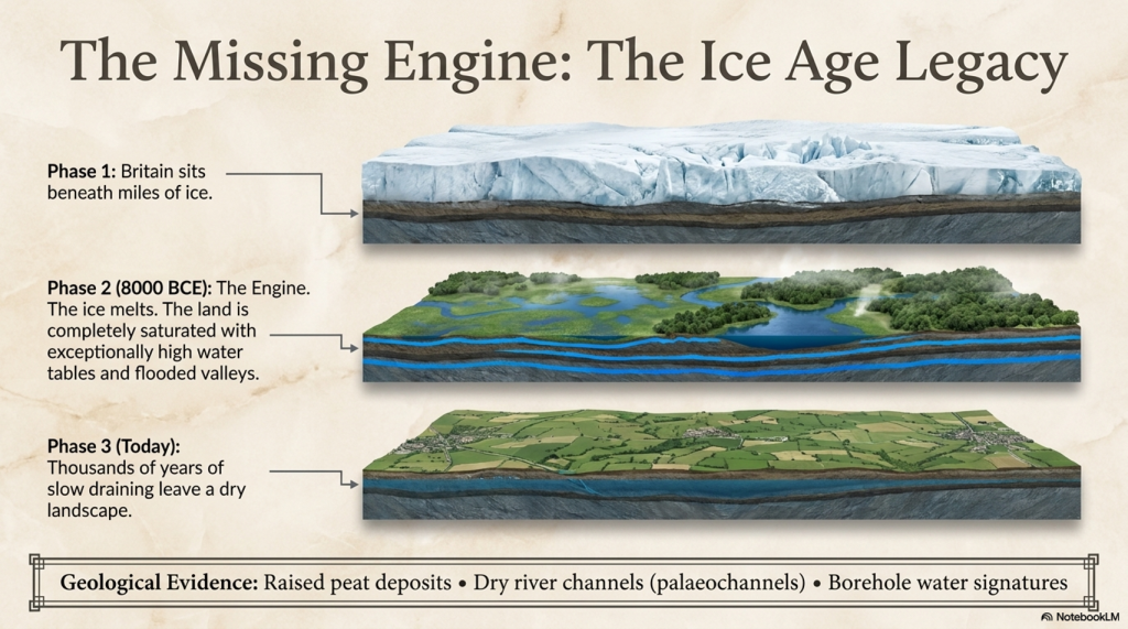
Roughly twenty-six thousand years ago, the Earth entered the final phase of the last ice age, when more than 30 million square kilometres of the northern continents were mantled by ice. Sea level dropped by over a hundred metres, continents expanded, and the atmosphere became drier and dustier. When the climate warmed, that frozen water returned to the ocean basins, transforming every river and shoreline on the planet. Understanding the magnitude and tempo of this transition is fundamental to reconstructing the landscapes that Holocene societies inherited. (The Post-Glacial Flooding Hypothesis)

The scientific history of sea-level research stretches back more than a century. Fairbridge (1961) first proposed that global “drowned terraces” recorded former sea levels. Oxygen-isotope analysis later provided a direct measure of global ice volume (Shackleton & Opdyke 1973; Chappell & Shackleton 1986). By the 1990s, uranium-thorium dating of coral reefs (Bard et al., 1990) and glacio-isostatic models (Lambeck & Chappell 2001) produced continuous global sea-level curves for the late Quaternary. Satellite altimetry and GRACE gravimetry now track present-day mass exchange between ice sheets and oceans with millimetre precision (Watkins et al., 2015; Cazenave et al., 2018).

These cumulative datasets reveal that the transformation from the Last Glacial Maximum (LGM) to the modern interglacial was neither instantaneous nor globally uniform. The following sections examine the evidence for the magnitude of the LGM, the deglacial rise in sea level, and the feedbacks that coupled ice, ocean, and atmosphere into a single dynamic system.

2. The Last Glacial Maximum

The LGM, dated between ~26 000 and 19 000 years BP, represents the maximum combined extent of Northern Hemisphere ice sheets. Reconstructions by Ehlers et al. (2018) show the Laurentide Ice Sheet extending south of the Great Lakes, the Fennoscandian complex covering Scandinavia, northern Britain, and the Baltic, and separate domes over the Barents and Kara Seas. In the Southern Hemisphere, the Patagonian, New Zealand, and Antarctic ice sheets expanded simultaneously. Global mean air temperature was about 5–6 °C lower than today (Tierney et al., 2020).

Cosmogenic-nuclide dating of moraines indicates near-synchronous maxima in both hemispheres within 1–2 kyr (Balco et al., 2009). Ice cores from Antarctica record atmospheric CO₂ concentrations of only ~190 ppm, the lowest of the last 800 kyr (Lüthi et al., 2008). The increased planetary albedo and reduced greenhouse forcing locked the Earth into a radiative imbalance until orbital precession increased summer insolation at high latitudes around 21 ka BP, initiating melting.

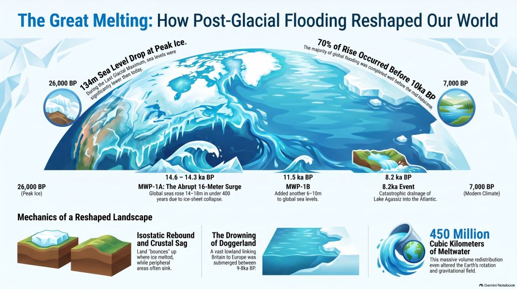
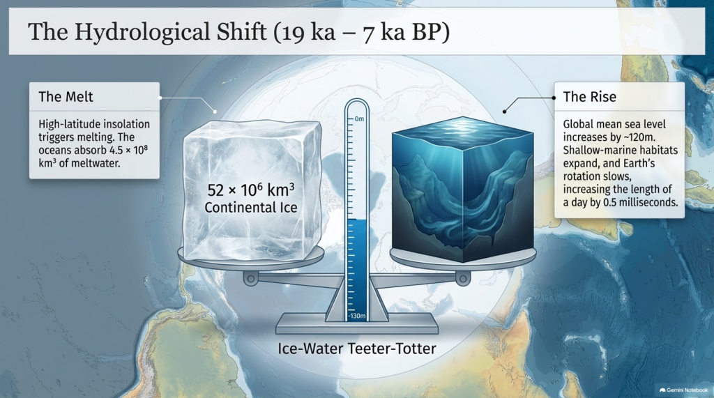
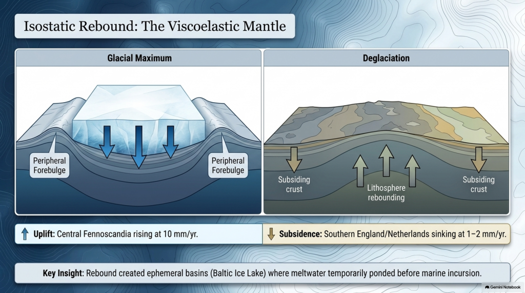
Sea level at the LGM stood 134 ± 5 m below present (Rohling et al., 2009; Lambeck et al., 2014), implying an extra ~52 × 10⁶ km³ of continental ice—roughly triple modern Antarctic volume. The load depressed the lithosphere by up to a kilometre and generated a peripheral forebulge hundreds of kilometres wide. When deglaciation began, these distortions created regional variations in relative sea level (RSL) of tens of metres—a problem that still complicates correlation between sites.

3. Quantifying Global Ice and Sea-Level Change

High-resolution oxygen-isotope records from the Red Sea (Rohling et al., 2009) and global benthic stacks (Lisiecki & Raymo, 2005) define the eustatic component of sea-level change. Grant et al. (2014) extended the Red Sea curve to 500 kyr BP and confirmed an approximately linear relation between δ¹⁸O and global mean sea level within ±140 m. Combined with coral-reef U/Th dates (Peltier & Fairbanks 2006) and glacio-isostatic modelling (ICE-6G v2; Peltier et al., 2015), these data yield the following deglacial sequence:

1. Stable minimum (26–19 ka) — Sea level constant near −130 m; ice volume at maximum.
2. Deglacial rise (19–7 ka) — Global mean increase ~120 m; average rate ~1.2 cm yr⁻¹.

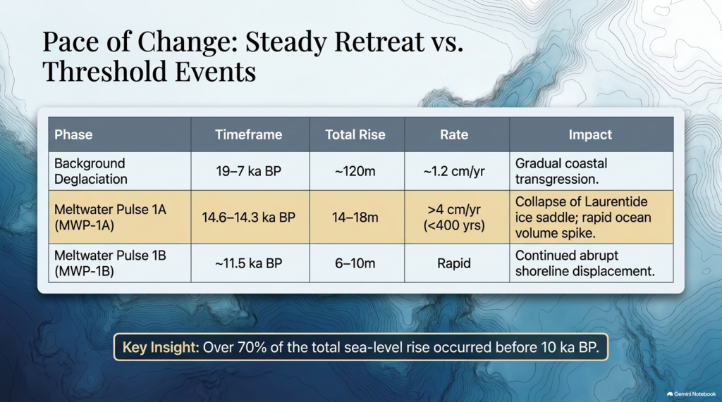
Waelbroeck et al. (2019) and Gowan et al. (2021) further improved resolution, showing that roughly 70% of the total rise occurred before 10 ka BP and that rates exceeded 4 cm yr⁻¹ during short meltwater pulses. These figures quantify the pace of global hydrological reorganisation that followed the LGM.

4. Meltwater Pulses and Deglacial Chronology

Superimposed on the long-term trend are several abrupt accelerations known as Meltwater Pulses (MWPs). MWP-1A (14.6–14.3 ka BP) raised global sea level by 14–18 m in < 400 years (Deschamps et al., 2012). Coral cores from Tahiti and Barbados capture the event as a distinct change in growth depth and isotope composition. MWP-1B, centred near 11.5 ka BP, added another 6–10 m (Liu et al., 2019). A later, smaller pulse (~8.2 ka BP) corresponded to catastrophic drainage of pro-glacial Lake Agassiz into the North Atlantic (Teller et al., 2002).

Numerical models (Gregoire et al., 2012) indicate that collapse of the Laurentide ice saddle triggered MWP-1A, releasing freshwater at ~0.3 Sverdrups—enough to disrupt the Atlantic Meridional Overturning Circulation (AMOC) and cause short-lived cooling across the Northern Hemisphere (Liu et al., 2009). Geomorphic evidence of megafloods, such as the Missoula outburst channels in North America (Bretz 1969; Baker 2013), provides analogues for the required discharge scale.

MWPs demonstrate that deglaciation was a series of threshold events rather than a steady retreat. The timing of pulses aligns closely with abrupt climatic shifts seen in Greenland ice cores (NGRIP Members 2004), underscoring the tight coupling between ice dynamics and global climate.

5. Isostatic Rebound and Crustal Adjustment

Once surface loads were removed, the lithosphere began to rebound. The process is governed by viscoelastic relaxation of the mantle with characteristic times of 1–5 kyr (Milne et al., 2006). Modern GPS and tide-gauge data show uplift of 10 mm yr⁻¹ in central Fennoscandia and subsidence of 1–2 mm yr⁻¹ in southern England and the Netherlands—the collapsing forebulge. Modelling (Lambeck et al., 2014; Peltier et al., 2015) reproduces these patterns when mantle viscosities of 3–5 × 10²¹ Pa s are used.

Rebound created ephemeral basins along glacial margins where meltwater ponded before marine incursion. The Baltic Ice Lake and the Champlain Sea are classic examples, forming as differential uplift temporarily dammed drainage routes (Saarnisto & Salonen 1995; Parent & Occhietti 1999). Many present-day estuaries owe their origins to these basins. Sediment cores from the Humber, Thames, and Rhine estuaries contain alternating freshwater and brackish layers that track the balance between isostasy and eustasy (Shennan et al., 2018).

6. The Rebirth of the Oceans

Between 19 ka and 7 ka BP, the oceans absorbed roughly 4.5 × 10⁸ km³ of meltwater, raising mean sea level by ~120 m. Coral records from Tahiti, Huon Peninsula, and the Sunda Shelf show a remarkably consistent transgression curve (Deschamps et al., 2012; Hanebuth et al., 2000). By 7 ka BP, sea level stabilised within a few metres of the modern datum.

The redistribution of this mass altered Earth’s rotation and gravitational field, increasing the length of day by 0.5 milliseconds (Mitrovica & Munk 2003) and displacing the geoid by several decimetres. More tangibly, flooding of continental shelves expanded shallow-marine habitats and enhanced nutrient exchange between land and sea, fuelling mid-Holocene marine productivity (Haug et al., 2001). The creation of new estuarine and lagoonal systems also provided nursery grounds for species that later became critical to human subsistence.

7. Climate Feedbacks During Deglaciation

Ice-core and modelling studies reveal that the deglacial rise in greenhouse gases both responded to and accelerated warming. CO₂ increased from 190 ppm at the LGM to 270 ppm by 11 ka BP (Lüthi et al., 2008). Methane doubled from 350 to 700 ppb (Loulergue et al., 2008). The combined radiative forcing of ~2.5 W m⁻² produced a global temperature increase of ~4 °C (IPCC AR6 2021). Shakun et al. (2012) demonstrated that Antarctic warming led the CO₂ rise by several centuries, implying that oceanic outgassing initiated the feedback loop.

Freshwater discharges into the North Atlantic weakened the AMOC and triggered millennial-scale climate reversals. The Younger Dryas (12.9–11.7 ka BP) involved a 5–7 °C drop in Greenland temperatures followed by rapid recovery within a few decades (Severinghaus et al., 1998). Numerical experiments show that such shifts require freshwater fluxes of 0.05–0.1 Sverdrups (Liu et al., 2009). Once meltwater routing shifted southward and AMOC strength recovered, interglacial stability was achieved.

8. The Transformation of North-West Europe

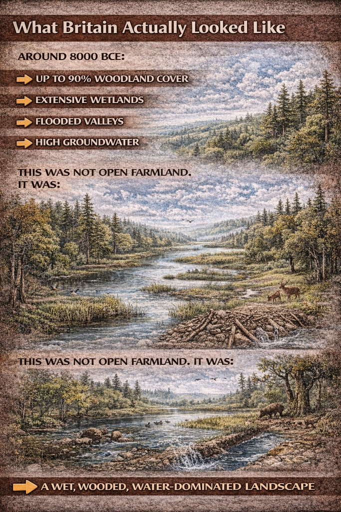
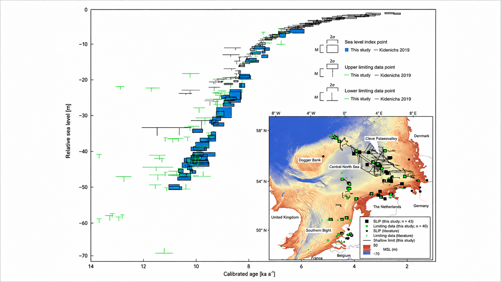
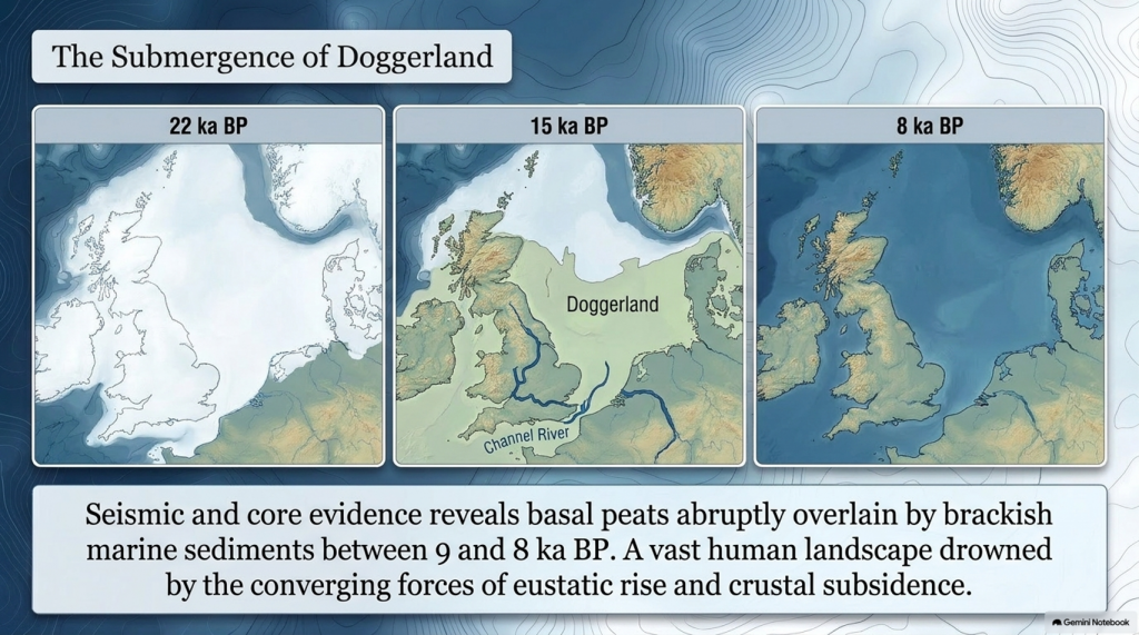
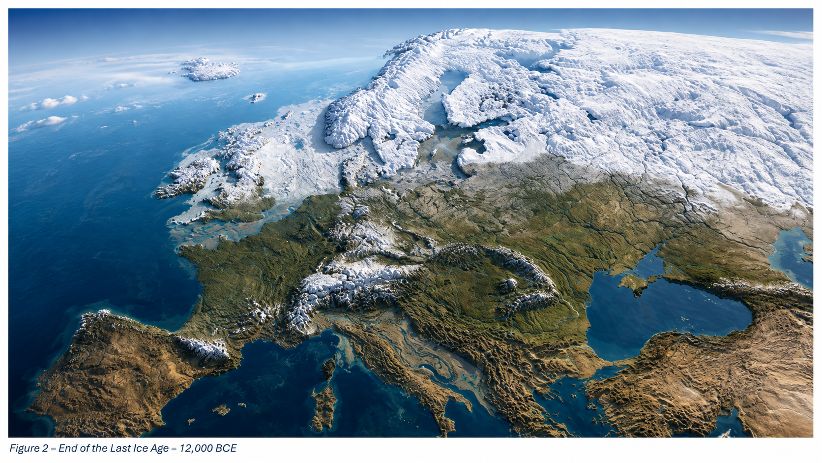
Retreat of the British–Irish Ice Sheet began near 22 ka BP and concluded by 15 ka BP (Clark et al., 2012). Deglaciation exposed outwash plains and periglacial lakes that evolved into estuaries and wetlands as sea level rose. Seismic and core evidence from the southern North Sea shows basal peats overlain by brackish and marine sediments between 9 and 8 ka BP (Hijma & Cohen 2011). These sequences chart the drowning of Doggerland—a vast lowland linking Britain to Europe. Pollen and macrofossil data indicate temperate woodland colonisation prior to submergence (Gaffney et al., 2009).

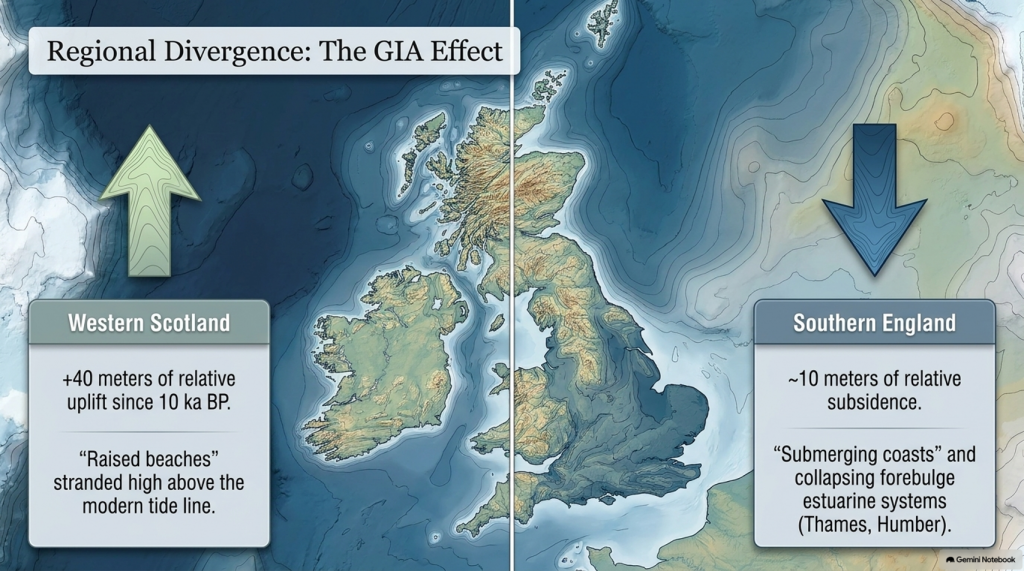
Regional RSL curves diverge sharply due to GIA: western Scotland has risen > 40 m since 10 ka, while southern England has subsided by ~10 m (Bradley et al., 2020). Raised beaches in the north and submerged forests in the south reflect this differential motion. In the English Channel, fluvial erosion during early deglaciation carved the “Channel River,” later flooded by 8 ka (Mellett et al., 2013). Similar sequences occur along the Irish and Danish coasts, documenting the progressive marine transgression of northwest Europe.

9. Towards a Global–Regional Synthesis

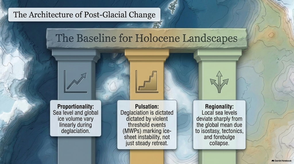
By combining isotopic, coral, and geodetic datasets, modern reconstructions achieve decimetre precision for Holocene sea level (Gowan et al., 2021). Three principles emerge:

1. Proportionality — Sea level and global ice volume vary linearly during deglaciation.
2. Pulsation — Superimposed meltwater pulses mark thresholds in ice-sheet stability.
3. Regionality — Local deviations result from isostasy, tectonics, and sediment compaction.

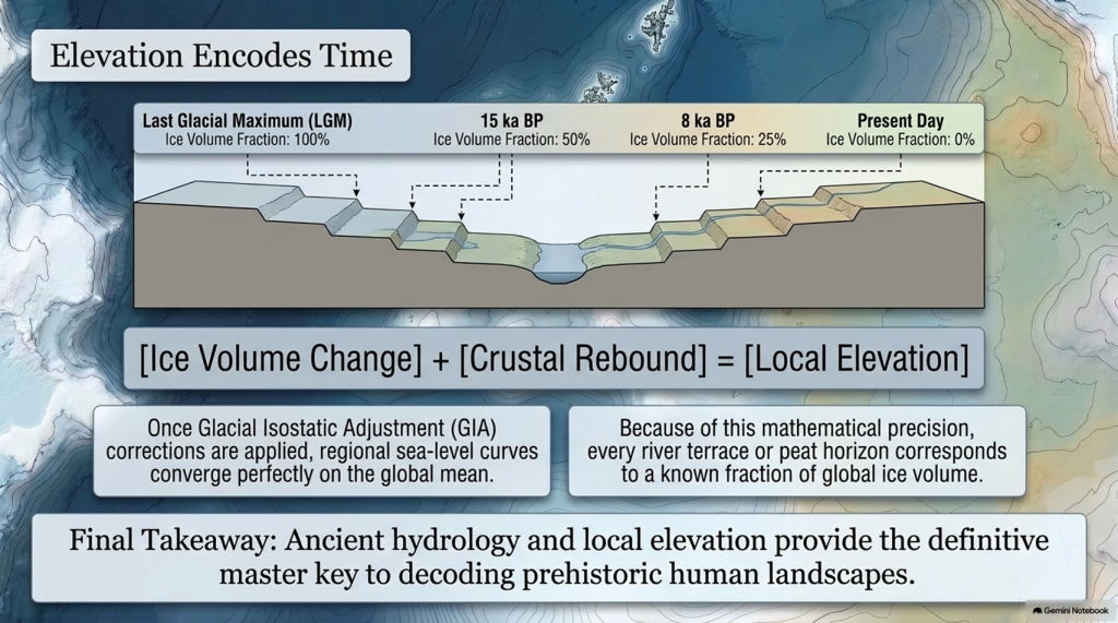
Shennan et al. (2018) synthesised over 500 Holocene RSL indicators for the British Isles, demonstrating that once GIA corrections are applied, regional curves converge on the global mean within analytical error. These findings provide a quantitative baseline for analysing river-terrace altitudes and groundwater histories in later chapters.

Equally important, comparison with modern sea-level observations highlights the extraordinary pace of contemporary change. Satellite altimetry records a mean rise of 3.4 ± 0.4 mm yr⁻¹ since 1993 (Cazenave et al., 2018)—an order of magnitude faster than the late-Holocene background rate (Kopp et al., 2016). The processes that ended the last ice age therefore remain relevant to current climate dynamics.

10. Conclusion

The end of the last ice age was a planetary event in which ice, water, and rock interacted on colossal scales. Between 26 ka and 7 ka BP, sea level rose more than 120 m, ice sheets vanished from most temperate latitudes, and the hydrological cycle intensified. The evidence—oxygen-isotope curves, coral terraces, basal peats, and glacio-isostatic models—forms a coherent narrative of gradual yet punctuated change.

These quantitative reconstructions define the environmental backdrop for all Holocene landscapes. They also establish a principle crucial to later chapters: that elevation within fluvial and coastal systems encodes time, because each terrace or peat horizon corresponds to a known fraction of global ice volume. The following chapter therefore turns from global physics to the mathematical description of flooding itself—the equations that translate ice-volume change into measurable hydrological response.

Plain-Language Conclusion

The ice age was like the planet putting a huge amount of the world’s water into giant freezers on land.  When those freezers started to melt:

• All that stored water went back into the oceans.
• The seas rose by about 120 metres.
• The weight of the ice came off the land, so some places bounced up, others sagged down.

Scientists can see this story in:

• tiny shells on the sea floor,
• old coral reefs now sitting at the “wrong” depths,
• layers of mud and peat around coasts.

Put simply:

We froze the oceans on land, then poured them back in. The combination of rising seas and bouncing crust rearranged coastlines everywhere, and we can measure it.

To read the rest of the book, follow this link: https://prehistoric-britain.co.uk/the-post-glacial-flooding-hypothesis-book

FREE ONLINE BOOK is available HERE: https://prehistoric-britain.co.uk/the-post-glacial-flooding-hypothesis-book

PODCAST

Author’s Biography

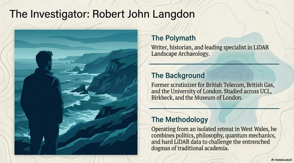
Robert John Langdon, a polymathic luminary, emerges as a writer, historian, and eminent specialist in LiDAR Landscape Archaeology.

His intellectual voyage has been interwoven with stints as an astute scrutineer in government and grand corporate bastions, a tapestry spanning British Telecommunications, Cable and Wireless, British Gas, and the esteemed University of London.

A decade hence, Robert’s transition into retirement unfurled a chapter of insatiable curiosity. This phase saw him immerse himself in Politics, Archaeology, Philosophy, and the enigmatic realm of Quantum Mechanics. His academic odyssey traversed the venerable corridors of knowledge hubs such as the Museum of London, University College London, Birkbeck College, The City Literature Institute, and Chichester University.

In the symphony of his life, Robert is a custodian of three progeny and a pair of cherished grandchildren. His sanctuary lies ensconced in the embrace of West Wales, where he inhabits an isolated cottage, its windows framing a vista of the boundless sea – a retreat from the scrutinising gaze of Her Majesty’s Revenue and Customs, an amiable clandestinity in the lap of nature.

Exploring Prehistoric Britain: A Journey Through Time

My blog delves into the fascinating mysteries of prehistoric Britain, challenging conventional narratives and offering fresh perspectives grounded in cutting-edge research, particularly LiDAR technology. I invite you to explore some key areas of my research. For example, the Wansdyke, often cited as a defensive structure, is re-examined in light of new evidence. I’ve presented my findings in my blog post Wansdyke: A British Frontier Wall – ‘Debunked’, and a Wansdyke LiDAR Flyover video further visualises my conclusions.

My work also often challenges established archaeological dogma. I argue that many sites, such as Hambledon Hill, commonly identified as Iron Age hillforts, are not what they seem. My posts Lidar Investigation Hambledon Hill – NOT an ‘Iron Age Fort’ and Unmasking the “Iron Age Hillfort” Myth explore these ideas in detail and offer an alternative view. Similarly, sites like Cissbury Ring and White Sheet Camp receive re-evaluations based on LiDAR analysis in my posts “Lidar Investigation Cissbury Ring through time” and “Lidar Investigation White Sheet Camp,“ revealing fascinating insights into their true purpose. I have also examined South Cadbury Castle, often linked to the mythical Camelot56.

My research also extends to ancient water management, including the role of canals and other linear earthworks. I have discussed the true origins of Car Dyke in multiple posts, including Car Dyke – ABC News Podcast and Lidar Investigation Car Dyke – North Section, which suggest a Mesolithic origin 2357. I also explore the misidentification of Roman aqueducts, as seen in my posts on the Great Chesters (Roman) Aqueduct. My research has also been greatly informed by my post-glacial flooding hypothesis, which has helped explain landscape transformations over time. I have discussed this hypothesis in several posts, including AI now supports my Post-Glacial Flooding Hypothesis and Exploring Britain’s Flooded Past: A Personal Journey

Finally, my blog also investigates prehistoric burial practices, as seen in Prehistoric Burial Practices of Britain and explores the mystery of Pillow Mounds, often mistaken for medieval rabbit warrens, but with a potential link to Bronze Age cremation in my posts: Pillow Mounds: A Bronze Age Legacy of Cremation? and The Mystery of Pillow Mounds: Are They Really Medieval Rabbit Warrens?. My research also includes astronomical insights into ancient sites, for example, in Rediscovering the Winter Solstice: The Original Winter Festival. I also review new information about the construction of Stonehenge in The Stonehenge Enigma.

Further Reading

For those interested in British Prehistory, visit www.prehistoric-britain.co.uk, a comprehensive resource featuring an extensive collection of archaeology articles, modern LiDAR investigations, and groundbreaking research. The site also includes insights and excerpts from the acclaimed Robert John Langdon Trilogy, a series of books that explore Britain during the Prehistoric period. Titles in the trilogy include The Stonehenge Enigma, Dawn of the Lost Civilisation, and The Post-Glacial Flooding Hypothesis, which offer compelling evidence of ancient landscapes shaped by post-glacial flooding.

To further explore these topics, Robert John Langdon has developed a dedicated YouTube channel featuring over 100 video documentaries and investigations that complement the trilogy. Notable discoveries and studies showcased on the channel include 13 Things that Don’t Make Sense in History and the revelation of Silbury Avenue – The Lost Stone Avenue, a rediscovered prehistoric feature at Avebury, Wiltshire.

In addition to his main works, Langdon has released a series of shorter, accessible publications, ideal for readers delving into specific topics. These include:

• The Ancient Mariners
• Stonehenge Built 8300 BCE
• Old Sarum
• Prehistoric Rivers
• Dykes, Ditches, and Earthworks
• Echoes of Atlantis
• Homo Superior
• 13 Things that Don’t Make Sense in History
• Silbury Avenue – The Lost Stone Avenue
• Offa’s Dyke
• The Stonehenge Enigma
• The Post-Glacial Flooding Hypothesis
• The Stonehenge Hoax
• Dawn of the Lost Civilisation
• Darwin’s Children
• Great Chester’s Roman Aqueduct
• Wansdyke

For active discussions and updates on the trilogy’s findings and recent LiDAR investigations, join our vibrant community on Facebook. Engage with like-minded enthusiasts by leaving a message or contributing to debates in our Facebook Group.

Whether through the books, the website, or interactive videos, we aim to provide a deeper understanding of Britain’s fascinating prehistoric past. We encourage you to explore these resources and uncover the mysteries of ancient landscapes through the lens of modern archaeology.

For more information, including chapter extracts and related publications, visit the Robert John Langdon Author Page. Dive into works such as The Stonehenge Enigma or Dawn of the Lost Civilisation, and explore cutting-edge theories that challenge traditional historical narratives.