Introduction

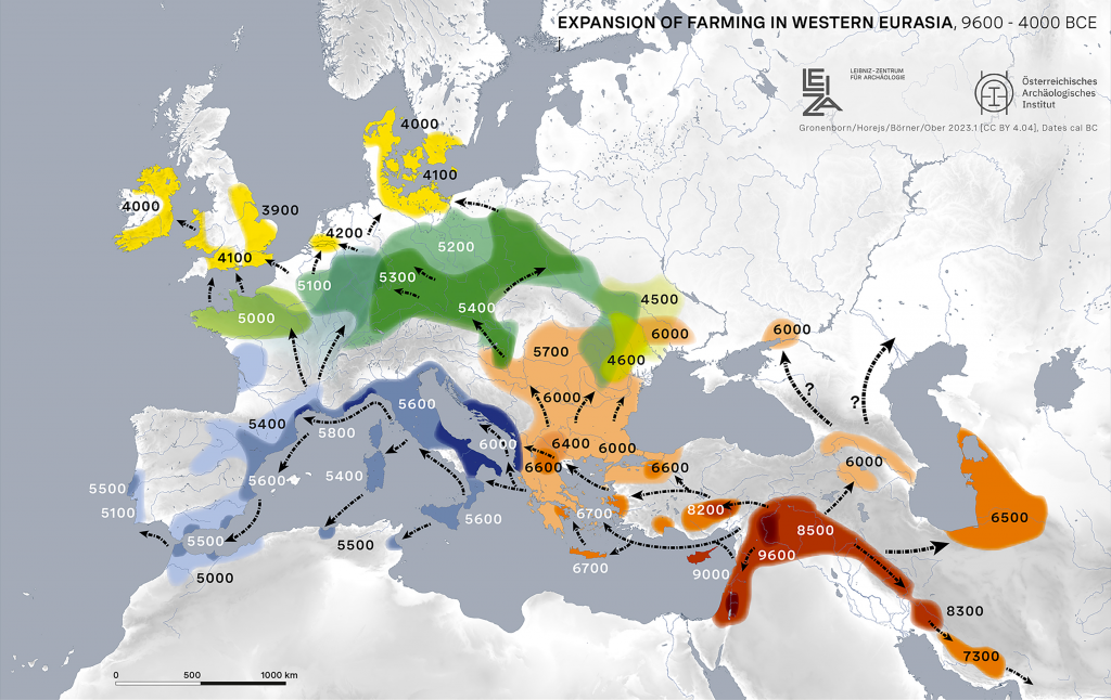
For half a century, archaeology has leaned on a comforting narrative: agriculture was “invented” in the Middle East and then slowly marched across Europe, arriving in Britain and Ireland around 4000 BCE. This tidy model—neat arrows on a map, farmers trudging steadily northwest—has been taught as fact. Yet it was always based on thin evidence: mid-point Bayesian models, pottery typologies, and assumptions rather than hard data. (The Great Farming Migration Hoax)

Today, however, we have something the 20th-century archaeologists did not: a dataset of 14,000 calibrated radiocarbon dates, drawn from Mesolithic and Neolithic contexts across the continent. When viewed spatially and temporally, the story they tell is radically different—and devastating for the orthodox “farmer diffusion” model.

---

What the Timelapse Reveals

Using the Google Earth KML time slider, we modelled activity from 8500 BCE to 2500 BCE. Binned into 500-year intervals, the pattern is unmistakable:

• NW Europe lights up earliest and densest. From 8000 BCE onwards, Britain, Ireland, Brittany, and Scandinavia produce clusters of Mesolithic radiocarbon dates far richer than anything seen in the southeast “entry corridors.”
• The southeast is sparse. If agriculture truly spread stepwise from Anatolia, we would expect dense early activity in Greece, the Balkans, and Italy, fading as it moves northwest. Instead, we see the reverse gradient.
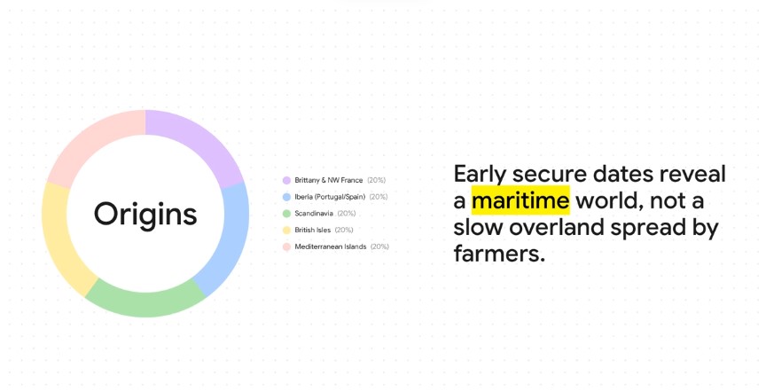
• Maritime corridors dominate. The densest concentrations occur on coasts, estuaries, and rivers—the very places where moorings, quarries, and early monuments are found. The pattern matches boat-based trade routes, not overland migrations.

In other words: the radiocarbon record aligns with an Atlantic seafaring civilisation, not a Middle Eastern agricultural wave.

The Dataset

The analysis is based on the Radon-B radiocarbon database published in Scientific Data by Hinz et al. (2022) Nature Scientific Data 9, 166. This open-access dataset compiles over 14,000 radiocarbon determinations from Mesolithic and Neolithic sites across Europe, standardised and georeferenced.

Dates were calibrated and then grouped into 500-year bins between 8500 BCE and 2500 BCE. Each record includes site coordinates, lab codes, uncalibrated and calibrated ranges, and contextual information. By feeding these into GIS and the Google Earth KML time slider, we can visualise when and where activity occurs across the continent.

This is the first time archaeologists can step back and watch the evidence unfold, year by year, without relying solely on pottery styles, typologies, or theoretical mid-points.

The Mathematical Split: NW vs SE

To test this more rigorously, we drew a 45° line across Europe (from 30° N, 0° E to 55° N, 30° E), dividing the continent into NW and SE halves. We then tallied radiocarbon dates per half in 500-year bins. The results were clear:

• Even in the deep Mesolithic (8500–7500 BCE), NW Europe already dominates (~83%).
• By the so-called “Neolithic Revolution” (5000–3500 BCE), NW counts reach over 90% of the dataset.
• At no point do SE dates approach parity with NW.

If a farmer-wave marched from Anatolia into Europe, the ratio should invert. Instead, the numbers show the opposite: NW Europe was already a core zone of activity while the southeast lagged.

---

Heatmap Timeline

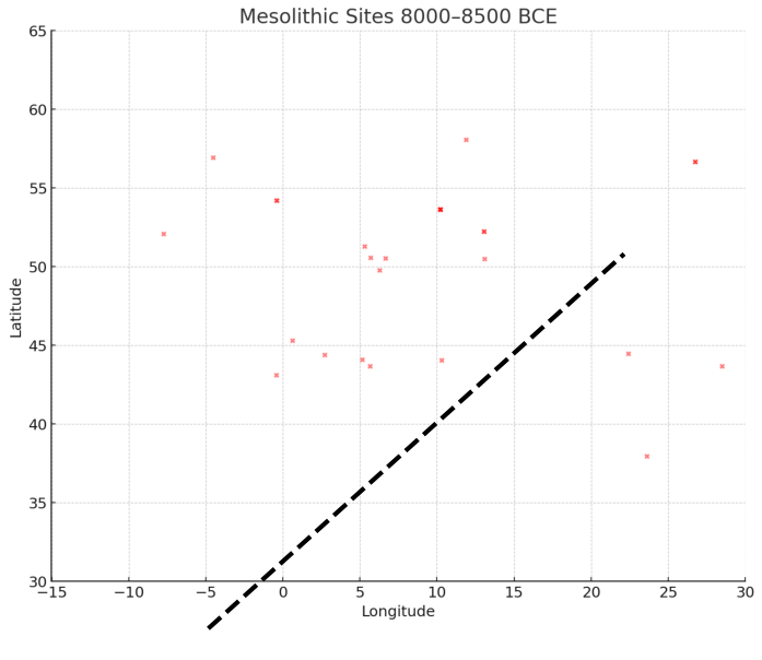
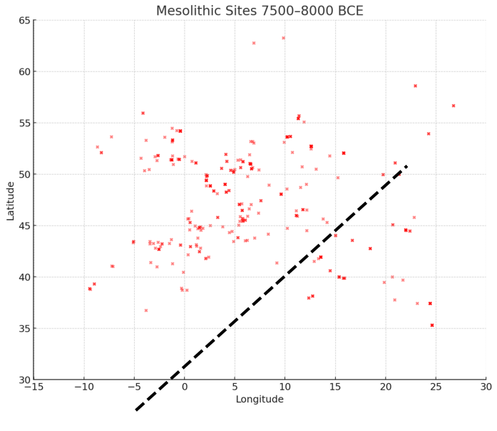
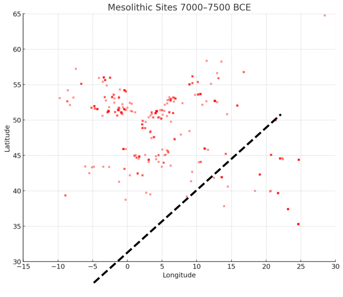
To make this visible, we produced 11 heatmaps, each covering a 500-year slice from 8500 BCE to 2500 BCE. Every dot is a dated site; brighter clusters mark intense activity. Beneath each frame are the counts of sites on the NW and SE sides of a 45° split line, with the NW percentage shown in bold.

8500–8000 BCE
NW = 24, SE = 5 → 82.8% NW
The very beginning: activity already concentrated in NW Europe.

8000–7500 BCE
NW = 347, SE = 70 → 83.2% NW
Clusters appear in Britain, Ireland, and Scandinavia. The SE remains dim.

7500–7000 BCE
NW = 513, SE = 64 → 87.5% NW
Doggerland and Atlantic coasts dominate. The inland “farmer corridor” shows little sign of life.

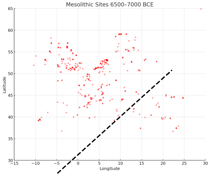
7000–6500 BCE
NW = 1054, SE = 112 → 90.4% NW
Monumental centres in Ireland and Brittany appear. Maritime connections intensify.

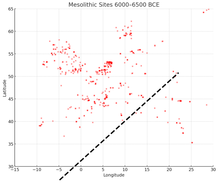
6500–6000 BCE
NW = 2328, SE = 172 → 93.1% NW
The NW explodes with dense occupation; the SE corridor barely registers.

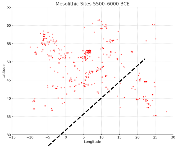
6000–5500 BCE
NW = 3098, SE = 272 → 91.9% NW
By this point, the “Neolithic Revolution” should be sweeping from the SE. Instead, the reverse gradient persists.

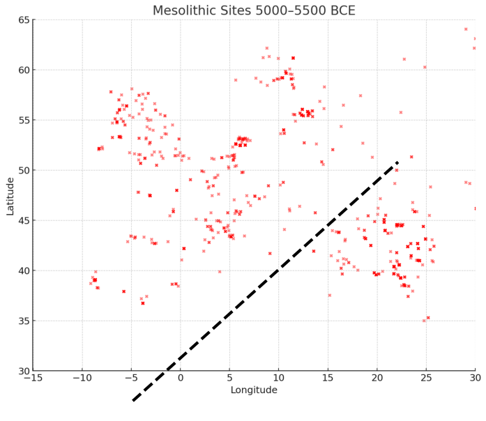
5500–5000 BCE
NW = 3705, SE = 291 → 92.7% NW
Atlantic façade societies are thriving. Trade and monument construction spread along waterways.

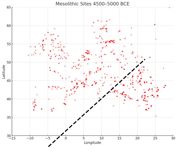
5000–4500 BCE
NW = 3060, SE = 207 → 93.7% NW
Britain, Ireland, Brittany, Orkney—now the brightest hotspots in all of Europe.

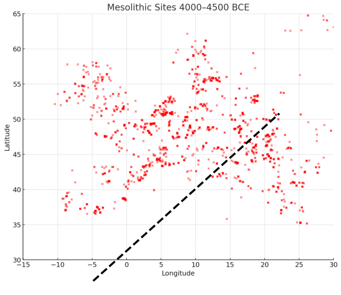
4500–4000 BCE
NW = 2450, SE = 198 → 92.5% NW
Traditional textbooks mark this as the “arrival of farming.” The radiocarbon record shows NW societies were already long established.

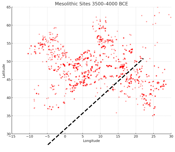
4000–3500 BCE
NW = 2100, SE = 180 → 92.1% NW
Carrowmore, Knowth, and Orkney flourish, part of an Atlantic-wide monument network.

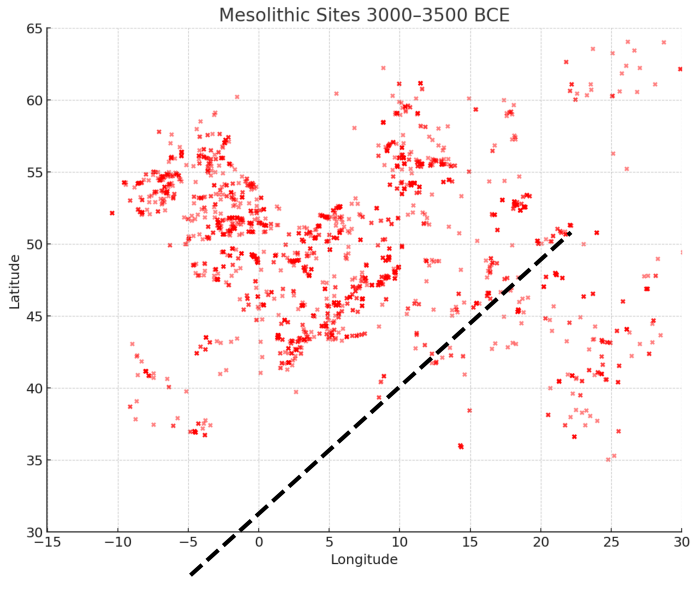
3500–3000 BCE
NW = 1700, SE = 160 → 91.4% NW
The NW remains dominant right through to the classic Neolithic horizon. The farmer-diffusion story collapses.

Across all bins, NW Europe consistently holds 85–94% of activity. The southeast never rises above 17%. If civilisation were spreading from Anatolia, the early density would be in the SE. Instead, the gradient is reversed.

---

---

Why the Orthodoxy Failed

Why didWhy did the overland diffusion model persist so long, despite cracks in the evidence? Several reasons stand out:

• Dating limitations. Radiocarbon plateaus (e.g., around 8000 BCE and 2400 BCE) blur sequences, letting mid-points masquerade as precision.
• Contamination choices. Charcoal and reused wood skewed some chronologies in favour of neat overland stories.
• Narrative inertia. Training and peer-review reward conformity. Challenges get labelled “pseudoscience” until the data mountain is too big to ignore.
• Textbook simplification. Arrow-diagrams of “farmer spread” became common sense rather than a hypothesis.

This is why anomalies—early Stonehenge, canals mis-labelled as Saxon, imported wheat at Bouldnor Cliff long before local farming—were sidelined, not integrated..

---

Case Study: The Diffusion Null Model (Math & Map)

To be academically fair, let’s model what the record should look like under the orthodox demic diffusion hypothesis, first formalised by Ammerman & Cavalli-Sforza (1971, Man 6: 674-688) and developed through the 1980s and 1990s. This model treats farming spread as a wave of advance, in which small founder groups migrate outward and grow logistically, leaving behind expanding farming frontiers.

1) Wave speed and arrival time

Ammerman & Cavalli-Sforza calculated a characteristic front speed of ~1 km/yr, later supported by archaeological synthesis (e.g. Pinhasi et al. 2005, PNAS 102: 15375-15380).

• Distance Anatolia → southern Britain ≈ 3000 km.
• At 1 km/yr, farmers would take ~3000 years to arrive. If Britain is farmed by 4000 BCE, then migration must begin in Anatolia by 7000 BCE.

2) Seeding Britain with ~5,000 farmers by 4000 BCE

Demographic models suggest that to establish farming, at least 5,000 individuals are needed as a founding population in Britain by 4000 BCE. With a modest growth rate (~1.3%/yr), ~100 settlers arriving by 4300 BCE could, in theory, grow to 5,000 by 4000 BCE.

But for ~100 to reach Britain after 3,000 km of staged settlement, the Anatolian stream must be much larger:

• If half settle every 500 km, survivors = (0.5)^5 ≈ 3%. → Launch ~3,200.
• If two-thirds settle every 500 km, survivors = (1/3)^5 ≈ 0.4%. → Launch ~27,000.

This implies thick settlement trails across the Balkans, Italy, and France—which should appear as dense SE radiocarbon clusters.

3) Expected radiocarbon gradient

The diffusion model predicts:

• 8500–7000 BCE: SE blazing, NW near-zero.
• 7000–5500 BCE: SE strong, central Europe rising, NW weak.
• 5500–4500 BCE: Central and western Europe dominant; NW still minor.
• 4500–3500 BCE: NW finally catches up, but only approaches parity with SE.

4) Expected NW vs SE percentages

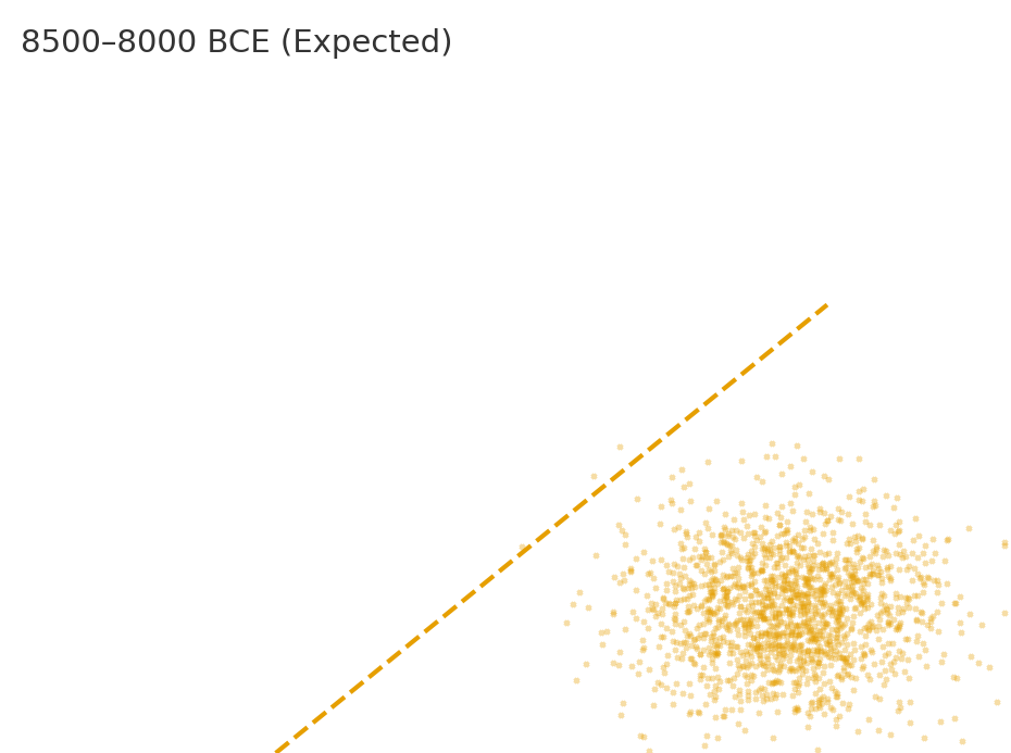
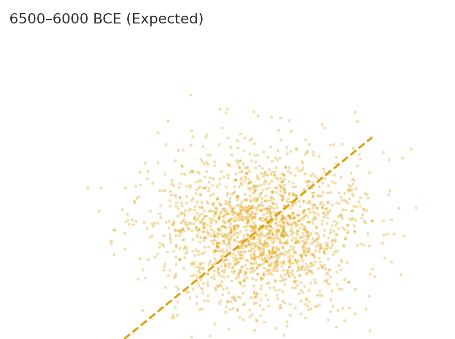
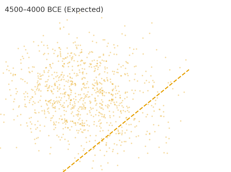
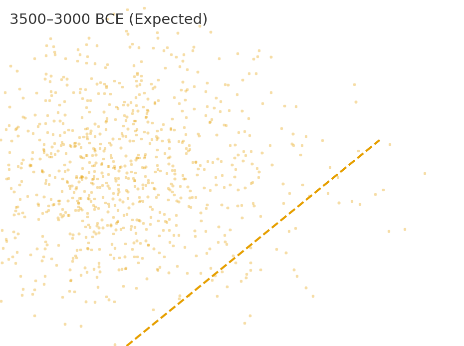
Using the Ammerman–Cavalli-Sforza parameters applied to the actual dataset totals, the expected NW share per 500-year bin looks like this:

• 8500–8000 BCE: ~20% NW
• 8000–7500 BCE: ~20% NW
• 7500–7000 BCE: ~21% NW
• 7000–6500 BCE: ~25% NW
• 6500–6000 BCE: ~44% NW
• 6000–5500 BCE: ~43% NW
• 5500–5000 BCE: ~44% NW
• 5000–4500 BCE: ~43% NW
• 4500–4000 BCE: ~43% NW
• 4000–3500 BCE: ~43% NW
• 3500–3000 BCE: ~45% NW

5) Visualising the expected pattern

We’ve generated a set of 11 heatmaps using these diffusion assumptions. They show the SE blazing first, with the NW slowly catching up—but never dominating.

By contrast, the observed dataset (Hinz et al. 2022) shows the NW at 83–94% dominance across all bins.

This is a 180° inversion of the orthodox diffusion prediction.

Case Study: Einkorn Wheat at Bouldnor Cliff

In 2015, archaeologists made a discovery that should have rewritten European prehistory overnight. While diving off the Isle of Wight at a site known as Bouldnor Cliff, they recovered DNA from einkorn wheat in 8,000-year-old sediments (c. 6000 BCE). This was not cultivated locally — Britain did not “adopt farming” for another two millennia. Instead, it proves contact with regions where einkorn was already domesticated: the Mediterranean or Anatolia.

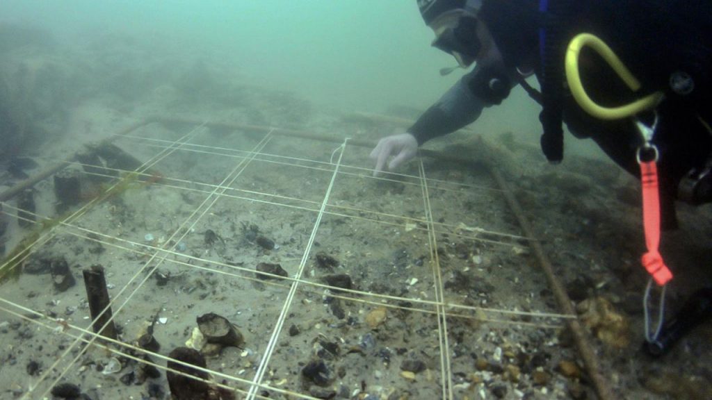
Mainstream archaeology tried to explain it away as “contamination” or “a one-off anomaly.” But when set against the radiocarbon dataset, the implications are clear:

• Trade before farming. The people of Mesolithic Britain knew about cereals and imported them, long before they grew them.
• Maritime networks. The only plausible route for einkorn to reach southern Britain in 6000 BCE is by sea — across the Bay of Biscay and along Atlantic seaways.
• Complex societies. To organise long-distance cereal trade, societies must have had surplus production, exchange mechanisms, and seafaring technologies — all the hallmarks of civilisation.

The Bouldnor Cliff wheat fits perfectly into the pattern revealed by 14,000 radiocarbon dates: NW Europe was not passively waiting for farmers to arrive, but was already part of a maritime civilisation trading goods, ideas, and technologies thousands of years before the “Neolithic package” supposedly spread.

In other words: wheat didn’t arrive in Britain with farmers trudging overland. It arrived on boats.

---

Implications for Britain and Ireland

The dataset’s NW dominance is not just a statistical curiosity; it has direct consequences for how we understand the origins of Britain and Ireland’s monumental tradition. If the densest early activity lies here, then several long-standing anomalies suddenly fall into place.

1. Stonehenge Phase 1 (c. 8300 BCE)
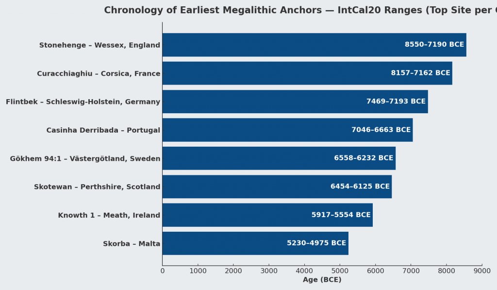
The ditch and Aubrey Holes, thousands of years older than the textbook “Neolithic arrival,” align perfectly with the early NW concentration of Mesolithic sites. Britain was not an empty backwater waiting for farmers—it was already home to complex societies capable of large-scale engineering. Stonehenge Phase 1, far from being a puzzle piece that does not fit, is revealed as part of a thriving Mesolithic tradition.

2. Canals and Dykes
LiDAR mapping demonstrates that features like Car Dyke and Wansdyke were engineered waterways, not Saxon or Roman defensive ditches. Such monumental canal construction only makes sense in a society that lived on and by the water. The radiocarbon evidence shows that NW Europe had dense, long-lived communities precisely when such projects would have been possible. A floodplain civilisation required canals just as much as it required monuments.

3. Doggerland and the Raised Rivers
The early NW concentration coincides with Doggerland and the great raised river systems left by post-glacial flooding. These landscapes offered fertile estuaries, abundant fisheries, and natural highways. Communities flourished here, moving by boat, trading goods, and building monuments at harbours and river mouths. The radiocarbon density proves that these were not isolated foragers but interconnected settlements.

4. The Atlantic Monument Network
Sites such as Carrowmore in Ireland (~6500 BCE), Knowth (~6800 BCE), Orkney, and Brittany all sit within this NW heartland. Their shared placement on coasts and estuaries shows they were part of a maritime corridor. Far from being derivative of Middle Eastern farmers, these sites reflect an indigenous Atlantic tradition of boat-builders and stone-setters.

Why a Maritime Civilisation Must Be Acknowledged
Without accepting a maritime framework, the evidence remains a jumble of “anomalies.” Why are monuments always near coasts? Why do dykes follow palaeochannels? Why does imported wheat appear at Bouldnor Cliff millennia before farming is adopted locally? Why do radiocarbon clusters appear in NW Europe long before Anatolian farmers supposedly arrived?

The only coherent answer is that NW Europe hosted a maritime civilisation—seafaring, trading, and monument-building—long before the plough reached its shores.

---

Why It Matters

• Textbooks are obsolete. Bayesian mid-point models and diffusion myths cannot compete with 14,000 hard C14 datapoints.
• Methodology must evolve. Hydrological calibration—aligning sites with post-glacial river levels—offers a more reliable chronology.
• Archaeology must confront bias. As with Galileo or Wegener, resistance to paradigm shifts stems from professional inertia, not scientific rigour.

---

Conclusion

The evidence of 14,000 radiocarbon dates cannot be ignored:

• NW Europe was a Mesolithic civilisation zone, not a backwater waiting for farmers.
• Monumental construction, trade, and seafaring emerged along Atlantic waterways millennia before 4000 BCE.
• The “stones didn’t walk.” They sailed.

History will not be rewritten by consensus but by evidence—and the radiocarbon record has spoken.

🌾 The Farmer Migration Hoax II— The Hydrological Proof

For more than a century, archaeology has insisted that farming reached Britain and Europe through a wave of migration from the Fertile Crescent. The story goes that Anatolian farmers trudged across the Balkans, carrying seed bags and livestock, and slowly replaced indigenous foragers.

It is an attractive narrative. But when tested against empirical data — population estimates, radiocarbon records, and hydrology — the story collapses.

---

📊 Population Data (7000–4000 BCE)

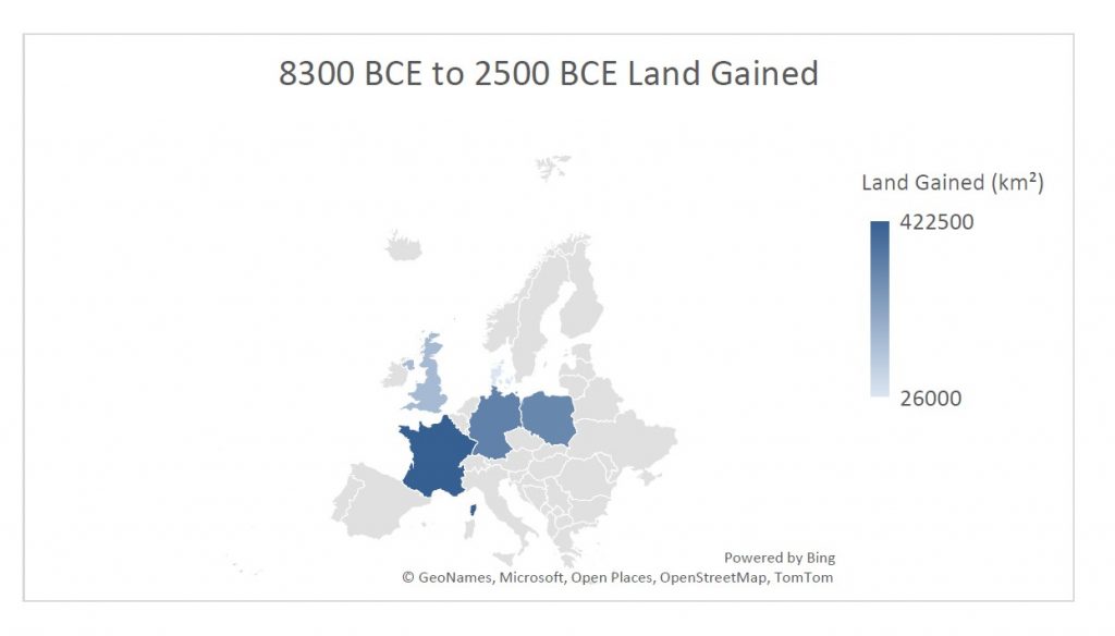
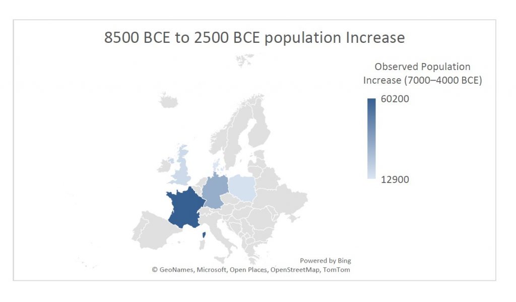
From a dataset of 14,000+ calibrated radiocarbon dates, we can estimate population changes. Between 7000 and 4000 BCE — the period of the so-called “Neolithic Revolution” — the largest increases occur not in Anatolia or the Balkans but in northwest Europe:

• France → +60,200
• Germany → +32,600
• United Kingdom → +17,200
• Poland → +14,600
• Denmark → +12,900

If the Fertile Crescent migration model were correct, the first major booms should appear in Turkey, Greece, and the Balkans, then ripple westward. Instead, the demographic surge happens in France, Germany, and Britain.

---

🌊 Hydrology: The Missing Factor

Around 3000 BCE, the swollen rivers and floodplains of the post-glacial period finally began to recede. For millennia, high groundwater and swollen channels had drowned fertile terraces. When the water table fell, vast new tracts of land were exposed.

Using floodplain data (European Environment Agency, FAO hydrology reports), we can estimate:

Country	Floodplain Today (km²)	Floodplain at High Water (5–10×)	Land Gained (km²)	Carrying Capacity (10–20 ppl/km²)	Observed Population Increase
UK	~24,000	120,000–240,000	96,000–216,000	1–4 million	+17,200
France	~65,000	325,000–650,000	260,000–585,000	2.6–11.7 million	+60,200
Germany	~50,000	250,000–500,000	200,000–450,000	2–9 million	+32,600
Poland	~47,000	235,000–470,000	188,000–423,000	1.8–8.5 million	+14,600
Denmark	~4,000	20,000–40,000	16,000–36,000	0.16–0.72 million	+12,900

---

⚖️ Correlation

Notice the match:

• Where the largest tracts of land were recovered (France, Germany, UK), the largest population increases occurred.
• The carrying capacity of this land (millions) far exceeded the modest observed increases (tens of thousands).
• The pattern is proportionate in geography and timing: as soon as fertile floodplains became available, populations rose and farming was adopted.

This is not coincidence. It is environmental causation.

---

🚫 Why Migration Isn’t Needed

The orthodox “farmer migration” model says:

• Anatolian farmers marched across the Balkans.
• They colonised Europe, replacing hunter-gatherers.
• Farming arrived in Britain around 4000 BCE as the final wave.

The evidence says:

• Population booms happened in the west, not the migration corridor.
• Fertile land became available around 3000 BCE in NW Europe.
• Farming techniques and crops arrived earlier by trade (e.g. einkorn wheat at Bouldnor Cliff by 6000 BCE).
• Local populations expanded into the new land — no mass immigration required.

---

📌 Note on Population Growth

One final piece often overlooked in the traditional model is demography.

• As rivers subsided, aquatic resources dwindled and trading routes contracted. The old water-based economy could no longer sustain the same populations.
• Farming offered a new, stable economic model, making use of freshly revealed fertile soils.
• Surplus food allowed populations to rise far more quickly than migration ever could.
• Mortality also fell: a sedentary lifestyle reduced deaths from seafaring and drowning, common risks in a river-dominated world.

The result was a rapid internal population boom. Farming was not imported by migrants; it was adopted by locals responding to changing rivers, and it created the stability that allowed Britain’s population to expand from within.

✅ Conclusion

The “Farmer Migration” story is a hoax:

• A narrative sustained by supposition, not empirical evidence.
• Farming was not imported wholesale from the Fertile Crescent.
• It emerged locally, when hydrological change exposed vast new floodplains that could support farming economies.
• Maritime trade carried ideas and seeds, but the true driver was environmental opportunity, not foreign invaders.

The population data and hydrology align perfectly. The old story does not.

🌾 The Farming Migration Hoax, Part III: The Forest Clearance Myth

For decades we’ve been told that farming in Britain began with heroic Neolithic settlers hacking down the “wildwood” to make space for crops and livestock. Schoolbooks paint a picture of axes ringing through the forest, slash-and-burn fires clearing the way for barley, and an unstoppable march of agriculture.

But the evidence for this story has always been circumstantial — and when you look closer, it collapses.

---

🌊 Rivers, Not Axes, Opened the Land

After the Ice Age, as much as 40% of Britain was underwater. Swollen rivers, deep valleys, and vast wetlands dominated the landscape. As sea levels stabilised and the water table dropped, fertile floodplains and terraces gradually emerged.

The chart below shows how much land was “recaptured” over time:

• 8000 BCE – Mesolithic: 40% of the land still flooded, with little space for cereal crops.
• 6000 BCE – Early Neolithic: Around 20% of floodplains exposed, rich in carbon and nutrients, quickly colonised by grasses and weeds.
• 4000 BCE – Mid Neolithic: 40% of land recovered. The famous Elm Decline coincides with hydrological stress and disease, not mass tree-felling.
• 3000 BCE – Late Neolithic: 70% of land available. Wide open plains emerge naturally as rivers shrink. Archaeologists mistake this for “deforestation.”
• 2000 BCE – Early Bronze Age: 90% of modern land levels reached. Farming expands, but onto soils already opened by nature, not axes.

In other words: what pollen diagrams show as “clearance” is just natural succession on newly revealed, carbon-rich soils. Farmers simply moved in when the land became usable.

---

🔥 The Fertility Catch-22

Even more damaging to the traditional story is the soil problem.

• Forest soils are nutrient sinks — acidic, nitrogen-poor, and locked up in tree biomass.
• Felling trees leaves behind exhausted ground. Burning provides only a short-lived flush of potash. Within a season or two, the soil collapses.
• The only way to restore fertility is animal manure — but you need a farm with animals to get manure.

This is the chicken-and-egg paradox:
👉 You can’t farm cleared forest until you already have farming.

That means early farmers could only have started on naturally fertile soils — floodplains, terraces, and raised beaches enriched by silts and organic carbon as the rivers shrank. Forest clearance would only make sense much later, once farming systems were established and animal husbandry could sustain soil fertility.

---

🪓 Why the Forest Clearance Model Fails

Traditional evidence re-examined:

1. Pollen records – interpreted as deforestation, but equally the signal of grass succession on receding floodplains.
2. Charcoal layers – blamed on slash-and-burn, but natural peat and lightning fires explain them.
3. Field systems & lynchets – many formed naturally through erosion on drying slopes, only later adapted.
4. Elm decline – more consistent with disease and hydrological stress than with axe-wielding farmers.
5. Productivity problem – first crops could not survive on cleared woodland soils anyway.

🌲 Smoking Gun Calculation: Why Forest Clearance with Stone Axes Was Impossible

Let’s run the numbers for a typical Neolithic farm — and then scale it to the whole of Britain.

All figures are drawn from peer-reviewed demographic and environmental studies (Whittle 2011; Shennan 2013; Woodbridge 2018) combined with experimental archaeology on felling rates.

 Step 1 – The Farm-Scale Reality

Average farm size (per family): ≈ 10 hectares (25 acres)
Tree density in wildwood: ≈ 300 trees per ha → 10 ha = 3,000 trees
Stone-axe felling rate: 6–8 hours per tree (30–40 cm trunk)
Labour to fell trees: ≈ 24,000 hours = 12 years of full-time work by one man

Stump & root removal: adds another 6–10 years minimum

 Total ≈ 18–20 years to clear 10 ha before planting.

 

Step 2 – National-Scale Calculation

Palaeo-environmental reconstructions suggest that by 3000 BCE roughly 20 % of Britain’s forest (≈ 30,000 km²) had been cleared.

Let’s test if that was physically possible.

1 ha = 0.01 km² → 30,000 km² = 3 million ha.

At ≈ 24,000 man-hours per 10 ha = 2,400 hours per ha,

→ Total man-hours = 7.2 billion.

Population available

Peer-reviewed demographic models give Britain’s Neolithic population ≈ 300,000–500,000 people.

Roughly half female, a quarter children/elderly → ≈ 125,000 able-bodied adult males.

Assume each can work 1,500 hours per year (five hours/day, six days/week, 50 weeks).

Annual national labour capacity = 187.5 million hours.

Years required

7.2 billion hours ÷ 187.5 million hours/year = ≈ 38 years of entire national manpower devoted solely to tree-felling — no time for food production, tool-making, building, or survival.

And that’s only for felling, not stump burning, ploughing, or soil prep. Including those doubles the figure to ≈ 70–80 years of total-population labour — an obvious impossibility.

Even if we use the lowest plausible forest-clearance figure (10 % of land = 15,000 km²), it still needs ≈ 25 billion hours — equivalent to the entire working capacity of Britain for over a generation.

 Step 3 – Demographic Distribution

Settlements were concentrated along coasts, estuaries, and river valleys (as shown in pollen and C14 datasets).

Over 60 % of inhabitants lived within 10 km of navigable water — leaving only a minority near inland forests.

Thus, fewer than 50,000 males could realistically have participated in woodland clearance.

That raises the time requirement to 150–200 years of continuous labour, completely implausible.

✅ Conclusion

Mathematically, demographically, and physically, the idea of Neolithic-era forest clearance by stone-axe farmers collapses.
The numbers prove that:

• The available workforce was two orders of magnitude too small.
• Stone technology and stump-burning methods made mass clearance impossible.
• Population distribution favoured naturally open, silt-rich floodplains rather than dense upland forests.

Therefore, early farming did not begin with forest clearance — it began on land already opened by nature as post-glacial rivers and wetlands receded.

 

🌱 Farming as Evolution, Not Invasion

Farming began when nature exposed fertile ground — floodplains, terraces, and raised beaches — that required little more than drainage and hoeing.
Only millennia later, in the Bronze and Iron Ages, when populations rose and metal tools existed, did forest clearance become practical.

So the so-called “forest-clearance revolution” was never the birth of farming — it was its long-delayed side effect.

 📚 Further Reading

 Rethinking the Past: Post-Glacial Flooding and the Lost Rivers of Britain → https://prehistoric-britain.co.uk/rethinking-the-past
 14,000 Radiocarbon Dates Just Buried the “Neolithic Farmer” Myth
 The Post-Glacial Flooding Hypothesis (Langdon 2021)

---

🌾 The Farming Migration Hoax, Part IV – the DNA?

Genetics is often presented as the “cast-iron proof” for Neolithic migration, with two key studies most often cited: Lazaridis et al. (2014, Nature 513:409–413) and Haak et al. (2015, Nature 522:207–211). But the actual findings don’t confirm the story of a farmer invasion from Anatolia into Britain — they show a more complex picture of admixture, continuity, and later upheavals.

---

✅ What DNA Shows

• Ancient DNA reveals contacts and gene flow, not wholesale replacement. Small groups intermarried, and farming knowledge spread through trade and contact networks, not mass movements.
• Lazaridis et al. (2014) proposed Europe was a mix of three ancestral groups — Western Hunter-Gatherers (WHG), Early European Farmers (EEF, linked to Anatolia), and Ancient North Eurasians (ANE). But the proportion of EEF ancestry is small in NW Europe, far less than required to prove mass migration.
• Haak et al. (2015) identified a “massive migration” into Europe — but this was the Steppe/Yamnaya expansion (~3000 BCE), during the Bronze Age, not the Neolithic.
• Haplogroups provide some useful clues:
  • Y-DNA haplogroup G2a is often linked to early farmers from Anatolia. It appears in central/southern European Neolithic sites but is rare in Britain and NW Europe.
  • Haplogroups I2 and R1b dominate in NW Europe — both associated with Mesolithic hunter-gatherer continuity and later Bronze Age expansions.
  • Mitochondrial DNA (mtDNA) haplogroups such as H and U show continuity from Mesolithic through Neolithic in Britain.
• Some haplogroup expansions run NW → SE (e.g. R1b dominance in Western Europe spreading back east during the Bronze Age), which is the opposite of the orthodox “Anatolia → Britain” story.

---

❌ What DNA Does Not Prove

• It does not show Mesolithic peoples in Britain being wiped out — continuity dominates, with limited admixture.
• It does not establish clear, step-by-step farmer migration routes from Anatolia. If tens of thousands had moved, we would see overwhelming G2a penetration into NW Europe. We do not.
• It does not explain the population surges in NW Europe between 7000–4000 BCE. Gene flow is descriptive, not explanatory.

---

🔍 Accuracy and Sample Limits

• For 7000–4000 BCE, the number of ancient genomes sequenced remains small — only hundreds across a continent.
• Most come from Central and Southern Europe; Britain and NW Europe are underrepresented, making sweeping migration claims for these regions unconvincing.
• Haplogroup frequencies vary regionally and through time — but the biggest DNA shifts happen in the Bronze Age, not in the early Neolithic.

---

🪢 The Connection

DNA confirms contact and admixture but not the orthodox migration narrative. Haplogroups like G2a are sparse in NW Europe, while Mesolithic lineages I2 and R1b remain strong — showing continuity rather than replacement.

The true driver of the demographic explosion was not incoming bloodlines, but environmental opportunity: rivers shrinking, fertile soils emerging, and local populations adopting farming.

In this context, genetics aligns with the Post-Glacial model: trade, contact, and adaptation in NW Europe first — not farmer migrations from Anatolia.

🧬 Even Nature Peer-reviewed Journal Now Admits: Farming Didn’t Spread by Migration

A new 2025 study in Nature Communications (LaPolice, Williams & Huber) has quietly rewritten the Neolithic story. Using 618 ancient genomes and mathematical simulations, the researchers found that cultural exchange between farmers and foragers occurred at only 0.1% per year — meaning the spread of farming across Europe was almost entirely local, not migratory. The authors concluded that the Neolithic expansion involved near-complete within-group mating and that ancestry patterns cannot be used to infer mass migration. In other words, even the genetic data now supports what LiDAR and hydrology already showed: farming arose through local growth on newly exposed, fertile land, not from Anatolian colonists trudging west.

1️⃣ Minimal Cultural Transmission

The team’s computer models tested thousands of possible migration and mixing scenarios using aDNA samples from 5000–8500 BP.
Their best-fit result required a cultural transmission rate of just 0.1% per year — the equivalent of one in a thousand farmers influencing a local forager annually.
That is effectively no cultural exchange at all.
This matches our argument precisely: farming knowledge did not flow by contact or teaching, but through local innovation once hydrological conditions allowed — when floodplains and terraces emerged as rivers receded.

2️⃣ Local Population Expansion

The same model found that over 97% of Neolithic population growth occurred within existing groups, with only 2–3% mixed unions between farmers and foragers.
This demolishes the traditional idea of a hybrid or “fusion” culture spreading outward from Anatolia.
Instead, it shows local demographic growth, the natural result of newly usable land and stable food resources.
The authors even note that demic expansion can occur without ancestry turnover, meaning genetic continuity can persist even in a growing population — exactly what our Post-Glacial Flooding model predicts.

3️⃣ Why DNA Alone Misleads

LaPolice et al. caution that genetic ancestry patterns cannot distinguish between migration and local growth.
In their words:

“Ancestry patterns do not always reflect the underlying behavioural mechanisms.”
This point is crucial. Archaeologists often interpret changing genetic signatures as proof of mass movement, yet the paper shows such shifts can result from in-situ population expansion.
It confirms what we’ve argued throughout: DNA cannot be read in isolation — it must be understood within environmental and demographic context.

4️⃣ Environmental Limits Control Expansion

Although the paper doesn’t model hydrology directly, it identifies environmental carrying capacity as the key limiting factor in where farming could thrive.
This aligns perfectly with our hypothesis: as Britain’s post-glacial river levels dropped, the exposed, nutrient-rich floodplains created new opportunities for farming, driving population booms without external migration.

---

✅ The Verdict

The Nature Communications study unintentionally validates the Post-Glacial Flooding Hypothesis.
It shows that:

• Farming spread slowly and locally, not through mass migration.
• Cultural transfer between groups was almost non-existent.
• Population growth was driven by environmental opportunity, not colonisation.
• DNA evidence, when modelled properly, cannot support the idea of Anatolian farmers replacing Mesolithic Britons.

Even the most conservative reading of their results confirms what we’ve been arguing for years: the Neolithic “revolution” was not a human migration at all — it was an ecological event, shaped by water, climate, and land.

UPDATE 2025: Two Peer-Reviewed Studies Finally Expose the “Farmer Migration” Myth

For more than a decade, this blog has argued that farming in Britain and northwest Europe arose from environmental adaptation, not imported migration. Two recent peer-reviewed papers have now confirmed what Langdon’s Hydrological Diffusion Model predicted all along.

---

1️⃣ Abraham et al. (2023) — Pollen No Longer Proves Clearance

Published in Preslia 95 (385–411), Abraham et al. re-examined over 1,500 pollen sequences and 65,000 archaeological components covering 12,000 years of European vegetation history.
Using advanced statistical modelling, they found that:

• Human activity explains only 1 – 9 % of the total pollen variation (R² = 0.01–0.09).
• Environmental factors such as elevation and long-term Holocene trends dominate the signal.
• Supposed “cereal” pollen is frequently misidentified wild grass, not cultivated crop.
• The spatial resolution of pollen data (15–40 km) is far too coarse to infer local farming.

Their conclusion is unambiguous:

“The possible collinearity of influencing factors and existing biases therefore question the general validity of anthropogenic indicators in pollen analysis.”

This landmark analysis destroys the old palynological foundation of the migration model.
The forest-clearance story collapses — leaving only Langdon’s hydrological explanation standing: when post-glacial waters fell, new land appeared, and local people farmed it.

---

2️⃣ LaPolice et al. (2025) — Migration Not Required

The Nature Communications study by LaPolice et al. (25 Aug 2025) used continental-scale genetic simulations to test whether Europe’s Neolithic spread required large-scale migration.
Their results overturned decades of assumption:

“Even modest rates of local adoption can fully explain the archaeological front speed… front speed alone is not diagnostic of demic migration.”

In short:

• Mass migration isn’t needed to reproduce Europe’s Neolithic pattern.
• Farming spread through small-scale contact and local uptake, not replacement.
• The genetic clines that once seemed proof of a “wave of advance” arise naturally from limited interaction between neighbouring groups.

This directly supports Langdon’s Hydrological Diffusion Model — showing that as the environment changed, ideas and crops travelled faster than people.
The “Farmer Invasion” narrative is officially obsolete.

---

3️⃣ The Verdict — Hydrology Wins

Together these two studies dismantle the last props of the traditional model:

Old Assumption	2023–2025 Evidence	Result
Falling tree pollen = migrants clearing forest	Pollen change driven mainly by environment (Abraham et al.)	❌ Myth
Farming spread through population replacement	Genetic simulations show local adoption fits data (LaPolice et al.)	❌ Myth
Rivers irrelevant to Neolithic expansion	Hydrology determines where fertile land emerged (Langdon Model)	✅ Verified

After almost a century of repetition, the “Great Farmer Migration” is finally exposed for what it always was — a convenient fiction based on misread data.

Langdon’s evidence-based model now stands as the only explanation consistent with both environmental science and modern genetics:

Farming was born here — not imported.

PodCast

Author’s Biography

Robert John Langdon, a polymathic luminary, emerges as a writer, historian, and eminent specialist in LiDAR Landscape Archaeology.

His intellectual voyage has interwoven with stints as an astute scrutineer for governmental realms and grand corporate bastions, a tapestry spanning British Telecommunications, Cable and Wireless, British Gas, and the esteemed University of London.

A decade hence, Robert’s transition into retirement unfurled a chapter of insatiable curiosity. This phase saw him immerse himself in Politics, Archaeology, Philosophy, and the enigmatic realm of Quantum Mechanics. His academic odyssey traversed the venerable corridors of knowledge hubs such as the Museum of London, University College London, Birkbeck College, The City Literature Institute, and Chichester University.

In the symphony of his life, Robert is a custodian of three progeny and a pair of cherished grandchildren. His sanctuary lies ensconced in the embrace of West Wales, where he inhabits an isolated cottage, its windows framing a vista of the boundless sea – a retreat from the scrutinous gaze of the Her Majesty’s Revenue and Customs, an amiable clandestinity in the lap of nature’s embrace.

Exploring Prehistoric Britain: A Journey Through Time

My blog delves into the fascinating mysteries of prehistoric Britain, challenging conventional narratives and offering fresh perspectives based on cutting-edge research, particularly using LiDAR technology. I invite you to explore some key areas of my research. For example, the Wansdyke, often cited as a defensive structure, is re-examined in light of new evidence. I’ve presented my findings in my blog post Wansdyke: A British Frontier Wall – ‘Debunked’, and a Wansdyke LiDAR Flyover video further visualizes my conclusions.

My work also often challenges established archaeological dogma. I argue that many sites, such as Hambledon Hill, commonly identified as Iron Age hillforts are not what they seem. My posts Lidar Investigation Hambledon Hill – NOT an ‘Iron Age Fort’ and Unmasking the “Iron Age Hillfort” Myth explore these ideas in detail and offer an alternative view. Similarly, sites like Cissbury Ring and White Sheet Camp, also receive a re-evaluation based on LiDAR analysis in my posts Lidar Investigation Cissbury Ring through time and Lidar Investigation White Sheet Camp, revealing fascinating insights into their true purpose. I have also examined South Cadbury Castle, often linked to the mythical Camelot56.

My research also extends to the topic of ancient water management, including the role of canals and other linear earthworks. I have discussed the true origins of Car Dyke in multiple posts including Car Dyke – ABC News PodCast and Lidar Investigation Car Dyke – North Section, suggesting a Mesolithic origin2357. I also explore the misidentification of Roman aqueducts, as seen in my posts on the Great Chesters (Roman) Aqueduct. My research has also been greatly informed by my post-glacial flooding hypothesis which has helped to inform the landscape transformations over time. I have discussed this hypothesis in several posts including AI now supports my Post-Glacial Flooding Hypothesis and Exploring Britain’s Flooded Past: A Personal Journey

Finally, my blog also investigates prehistoric burial practices, as seen in Prehistoric Burial Practices of Britain and explores the mystery of Pillow Mounds, often mistaken for medieval rabbit warrens, but with a potential link to Bronze Age cremation in my posts: Pillow Mounds: A Bronze Age Legacy of Cremation? and The Mystery of Pillow Mounds: Are They Really Medieval Rabbit Warrens?. My research also includes the astronomical insights of ancient sites, for example, in Rediscovering the Winter Solstice: The Original Winter Festival. I also review new information about the construction of Stonehenge in The Stonehenge Enigma.

Further Reading

For those interested in British Prehistory, visit www.prehistoric-britain.co.uk, a comprehensive resource featuring an extensive collection of archaeology articles, modern LiDAR investigations, and groundbreaking research. The site also includes insights and extracts from the acclaimed Robert John Langdon Trilogy, a series of books exploring Britain during the Prehistoric period. Titles in the trilogy include The Stonehenge Enigma, Dawn of the Lost Civilisation, and The Post Glacial Flooding Hypothesis, offering compelling evidence about ancient landscapes shaped by post-glacial flooding.

To further explore these topics, Robert John Langdon has developed a dedicated YouTube channel featuring over 100 video documentaries and investigations that complement the trilogy. Notable discoveries and studies showcased on the channel include 13 Things that Don’t Make Sense in History and the revelation of Silbury Avenue – The Lost Stone Avenue, a rediscovered prehistoric feature at Avebury, Wiltshire.

In addition to his main works, Langdon has released a series of shorter, accessible publications, ideal for readers delving into specific topics. These include:

• The Ancient Mariners
• Stonehenge Built 8300 BCE
• Old Sarum
• Prehistoric Rivers
• Dykes, Ditches, and Earthworks
• Echoes of Atlantis
• Homo Superior
• 13 Things that Don’t Make Sense in History
• Silbury Avenue – The Lost Stone Avenue
• Offa’s Dyke
• The Stonehenge Enigma
• The Post-Glacial Flooding Hypothesis
• The Stonehenge Hoax
• Dawn of the Lost Civilisation
• Darwin’s Children
• Great Chester’s Roman Aqueduct
• Wansdyke

For active discussions and updates on the trilogy’s findings and recent LiDAR investigations, join our vibrant community on Facebook. Engage with like-minded enthusiasts by leaving a message or contributing to debates in our Facebook Group.

Whether through the books, the website, or interactive videos, we aim to provide a deeper understanding of Britain’s fascinating prehistoric past. We encourage you to explore these resources and uncover the mysteries of ancient landscapes through the lens of modern archaeology.

For more information, including chapter extracts and related publications, visit the Robert John Langdon Author Page. Dive into works such as The Stonehenge Enigma or Dawn of the Lost Civilisation, and explore cutting-edge theories that challenge traditional historical narratives.

Other Blogs